Weather Research and Forecasting Model simulations of extended warm-season heavy precipitation episode over the US Southern Great Plains: data assimilation and microphysics sensitivity experiments

Figures & data

Fig. 1 Location map. Boundaries enclose WRF-ARW outer model domain, with thick broken line delineating the inner 3-km grid spacing nested domain centred over the Southern Great Plains (SGP) Central Facility (CF). Dark (light) dotted square surrounding the CF demarcates 9×9 (35×35) grid points over which model results and derived statistics were averaged. Locations are given for SGP Surface Meteorological Observation System (SMOS) instruments (red crosses) and CF rawinsonde station (centre of star) used for data assimilation (DA), and for WSR-88D radar at Vance AFB (green asterisk) used for comparison.

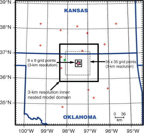
Table 1. Particle size distribution (PSD) characteristics employed for simulated radar experiments

Experiment or microphysics scheme	Water species	Functional form	N 0/intercept parameter	λ (slope)	m(D)=αD ^β or constant density	Remarks	References
Cloud	Monodisperse	N c=1×10^8		Spherical particles with	^R1 Rutledge and
Rain	Exponential	8×10^6	Diagnosed	ρ w	constant density	Hobbs (1983)
Lin	Snow	Exponential	3×10^6	Diagnosed	ρ s=100
Graupel	Exponential	4×10^4	Diagnosed	ρ g=400
Ice*	Monodisperse	N i from A13 of R1
Cloud	Monodisperse	N c=3×10^8		ρ w	Mass-dependent ice	^R2 Hong et al. (2004)
Rain*	Exponential	8×10^6	Diagnosed	ρ w	concentration
WSM5	Snow*	Exponential	Eq. 6 of R2	Diagnosed	ρ s=100
Graupel	NOT	USED
Ice*	Monodisperse	N i from Eq. 5c of R2		α=1/11.9^2, β=2
Cloud*	Monodisperse	N c=1×10^8		ρ w	Mass-Lookup table	^R3 Houze et al. (1979)
Rain*	Exponential	Rain content dependent		ρ w	based on R3
Eta	Snow*	Exponential	Lookup table based on R3
Graupel	NOT	USED
Ice	NOT	USED
Cloud	Same as WSM5				Temperature dependent
Rain*	Same as WSM5				snow intercept
WSM6	Snow*	Same as WSM5				parameter as in WSM5
Graupel	Exponential	4×10^6	Diagnosed	ρ g=500
Ice*	Same as WSM5
Cloud	Monodisperse	N c=1×10^8		ρ w	Spherical particles with	^R4 Thompson
Rain	Exponential	8×10^6	Diagnosed	ρ w	constant diameter	et al. (2008)
Goddard	Snow	Exponential	1.6×10^7	Diagnosed	ρ s=100
Graupel	Exponential	4×10^6	Diagnosed	ρ g=400
Ice*	Monodisperse	N i from A13 of R1
Cloud*	Generalised gamma	N c=3×10^8	Eq. A4 of R4	ρ w	Number concentrations for rain and ice are	^R5 Morrison et al. (2009)
Rain*	Exponential	Eq. 3 of R5	Diagnosed	ρ w	predicted
Thompson	Snow*	Eq. 1 of R4	Parameters from R6		α=0.069, β=2
Graupel*	Exponential	Mixing ratio-dependent (R4)		ρ g=400	^R6Field et al. (2005)
Ice*	Exponential	Eq. 3 of R5	Diagnosed	ρ i=890
Cloud*	Generalized gamma	Diagnosed	Eq. 2 of R7 (νc=1, α c=3)	ρ w	Number concentrations for cloud and rain are	^R7 Lim and Hong (2010)
Rain*	Generalized gamma	Diagnosed	Eq. 2 of R7 (νr=2, α r=1)	ρ w	predicted
WDM5	Snow*	Exponential	Eq. 6 of R2	Diagnosed	ρ s=100
Graupel	NOT USED
Ice*	Same as WSM5
Cloud*	Same as WDM5
Rain*	Same as WDM5
WDM6	Snow*	Same as WDM5
Graupel	Same as WDM5
Ice*	Same as WDM5

For all microphysics-based experiments, the PSDs are used for weather (S-band) and cloud (Ka-band) radar reflectivity simulations. ρ _w is the density of water (1000 kg m⁻³), and ρ _s and ρ _g are densities of snow and graupel, respectively. The * in the Water Species column indicates the relevant QuickBeam routines for the corresponding condensate were modified or replaced by code snippets from the WRF-ARW microphysics routines to implement WRF-ARW-consistent microphysical attributes. R1–R7 in centre of table indicate references given in the extreme right-hand column. See text for further details.

Table 2. Root mean-squared error (RMSE, dBZ) and mean error (ME, dBZ) for eight WRF microphysics simulations of radar reflectivity with (OBNUD, 3DVAR, 4DVAR) and without (CNTRL) data assimilation (DA) for 0600 UTC 27 May–1800 UTC 31 May, 2001 (108-hourly verifications)

		Data assimilation (DA)
		CNTRL		OBNUD		3DVAR		4DVAR
Microphysics		RMSE	ME	RMSE	ME	RMSE	ME	RMSE	ME
Lin	All times	26.4	14.1	26.7	14.6	17.5**	11.1*	22.5	11.8
Initial DA	28.2	16.2	28.5	16.7	16.4**	9.3**	24.2	12.1*
WSM5	All times	18.9	11.4	20.7***	13.9***	17.6	11.7	20.1*	13.7***
Initial DA	20.7	13.8	22.1*	15.8**	18.8*	12.1*	21.8	15.9***
Eta	All times	21.1	12.8	22.2	13.7	17.6***	10.6***	19.2**	10.8***
Initial DA	22.9	15.8	24.0	16.8	14.7***	9.0***	20.7*	12.7**
WSM6	All times	24.2	15.3	24.8	16.2	18.9***	12.5***	24.1	14.9
Initial DA	26.1	18.3	26.7	18.9	20.7***	14.7***	25.5	17.9
Goddard	All times	22.3	15.6	21.2	15.2	19.8**	13.8***	20.4*	14.4**
Initial DA	24.1	17.8	22.8	16.8	21.7*	15.6***	22.5	16.4*
Thompson	All times	18.9	12.4	19.2	11.1**	17.5***	10.1***	17.8***	10.5***
Initial DA	19.3	12.9	20.1	10.6**	18.0*	10.1***	16.7***	9.2***
WDM5	All times	18.0	10.7	19.6**	12.1**	14.7***	6.8***	18.0	9.6
Initial DA	19.6	12.8	20.6	13.5	16.2***	8.4***	19.8	11.4
WDM6	All times	23.1	12.9	24.6	14.4	15.8**	7.3***	22.2	12.0
Initial DA	25.0	15.9	26.5	17.5	16.4***	7.2***	24.2	15.2

Same statistics also were computed for the first 36 h of the data assimilation to assess the immediate data assimilation effects (Initial DA, 36-hourly verifications). To express ME in dBZ, the average departures from the observation (ME_d in mm⁶ m⁻³) were equated to 0 for small departure values between −1 and +1, given by 10*log10(ME_d) for ME_d>1, and given by −10*log10 (−ME_d) for ME_d<−1. Bold values indicate OBNUD, 3DVAR and 4DVAR RMSEs and MEs for which their differences from the corresponding CNTRL values are statistically significant at levels of ≤1% (triple asterisks), ≤5% (double asterisks) and ≤10% (single asterisk) according to a two-tailed ordinary bootstrap test (Section 2.3).

Fig. 2 SGP surface and rawinsonde observations used in the data assimilation (DA) experiments. Upper panels depict surface measurements across Oklahoma and southern Kansas at (a) 0600 and (b) 1200 UTC 27 May 2001. Bottom panel (c) contains rawinsonde observations at the CF for 0600 (red) and 1200 (blue) UTC 27 May 2001. Surface measurements plotted in (a) and (b) are dry-bulb (red) and dew point (green) temperatures (°C), station pressure (hPa, purple), winds (m s⁻¹; full barb indicates 5 m s⁻¹) and pressure tendency (signed) in preceding 3 hours (in 0.1 hPa; black). Relative humidity values also are shown as substitutes for cloud (1 octa equivalent to 12.5% RH; shaded circle). In (c), air temperatures (solid lines) and dewpoints (dashed lines) are in °C; winds are in m s⁻¹, with full barb indicating 5 m s⁻¹ and solid flag 25 m s⁻¹.

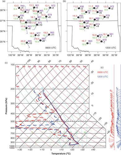
Fig. 3 Spatial (left) and temporal (right) convection signatures over the Southern Great Plains (SGP) for 27–31 May 2001. (a) EOF1 (dimensionless) and (b) mean (shading, dBZ) and frequency (>10 dBZ, contours,%) of WSR-88D weather radar (Vance AFB, Fig. 1) reflectivity for the inner 3-km grid spaced model domain in Fig. 1 (thick broken line). (c) Time coefficients of EOF1 in (a) (standardised and scaled, red line) and hourly precipitation rates from surface meteorological observation stations (bars, mm). (d) Millimeter cloud radar reflectivity (dBZ) at the CF (located by white squares in (a), (b); from Mace et al. 2006) and (e) CF liquid (below 4 km) and ice (above 4 km) water concentration (g m⁻³) obtained via Mace et al. (2006). Letters A, B, C at top of (c) identify convective events at corresponding times (day/hour bottom abscissa). Parts of the extended low-level MMCR radar echoes below 3 km likely are contaminated by radar signals from non-cloud sources.

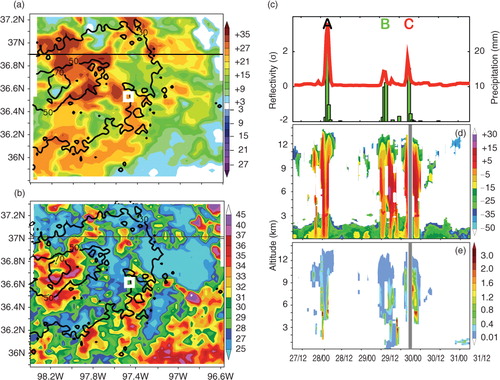
Fig. 4 Spatial (shading) and corresponding temporal (time series) characteristics of simulated weather radar reflectivity fields over the Southern Great Plains (SGP) for the inner 3-km grid spaced model domain (Fig. 1, thick broken line) for eight WRF microphysics experiments with no data assimilation (DA) (CNTRL) for 27–31 May 2001. Columns 1 and 3 contain EOF1 patterns (dimensionless, colour shading, arbitrary scale at bottom) and frequency of intensity (above 10 dBZ, black contours,%) of simulated reflectivity for the microphysics-based PSD simulations (Table 1). Columns 2 and 4 contain time series of scores (blue) corresponding to the EOF1 patterns in columns 1 and 3, respectively. For columns 2 and 4, the colour coding for the above time series appears at the top, along with that for a counterpart time series for EOF1 of the WSR-88D reflectivity observations (red) derived from Fig. 3a and c. All EOF time series are standardised (σ in units of mm⁶ m⁻³) and scaled by 100. Black squares in columns 1 and 3 show location of SGP Central Facility (CF).

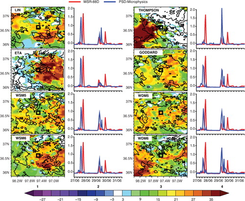
Fig. 5 Simulated cloud radar reflectivity profiles for 27–31 May 2001 (dBZ, colour scale at bottom) for eight WRF microphysics schemes for the following experiments: (a) no data assimilation (DA) (CNTRL), (b) observational nudging analysis (OBNUD), (c) three-dimensional variational DA (3DVAR) and (d) four-dimensional variational DA (4DVAR). Cloud radar reflectivity values were averaged over the 9×9 grid points nearest to the SGP CF (Fig. 1, dark dotted square). Middle row shows the MMCR-observed cloud radar reflectivity Best Estimate for the CF, with colour arrows indicating observed convective events A (black), B (green) and C (red) in Fig. 3c–e. WSM5(6) and WDM5(6) are WRF Single-Moment 5(6)-class and WRF Double-Moment 5(6)-class microphysics schemes, respectively. Parts of the extended low-level MMCR radar echoes below 3 km likely are contaminated by radar signals from non-cloud sources.

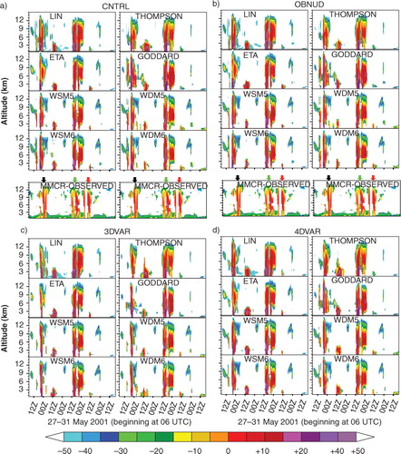
Fig. 6 Contributions (%) of individual hydrometeor species (colours, coded at top) to total simulated cloud radar reflectivity for eight WRF microphysics CNTRL simulations in Fig. 5a at five representative altitudes (1, 3, 5, 7 and 9 km) for 27–31 May 2001. Simulated cloud radar reflectivity was computed using particle size distribution (PSD) characteristics for individual microphysics schemes (Table 1), and averaged over the 9×9 grid points nearest to the SGP CF (Fig. 1, dark dotted square). For Eta microphysics, snow and ice are not differentiated. WRF single/double-moment five-category scheme (WSM5/WDM5) provides explicit treatment of cloud water, rainwater, snow and ice species. Lin, WSM6, WDM6, Goddard and Thompson microphysics schemes predict the additional graupel species. Black (A), green (B) and red (C) arrows at top indicate the three organised convective events identified in Fig. 3c–e and 5 (middle row). Finite but numerically negligible (<1e–10 kg/kg) rain mixing ratios are generated below 3 km outside the three precipitation events A, B and C in the Lin simulation, which affected the reflectivity percentage contributions when only rainwater is simulated at a given instant of time.

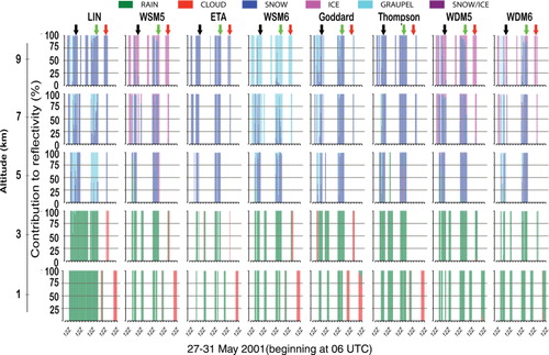
Fig. 7 Vertical profiles of correlations (values along bottom abscissa) between simulated and MMCR-observed cloud radar reflectivity for 27–31 May 2001 for eight WRF microphysics schemes for the following experiments (colour-coded at bottom): no data assimilation (DA) (CNTRL; dark blue), observational nudging analysis (OBNUD; green), three-dimensional variational DA (3DVAR; light blue) and four-dimensional variational DA (4DVAR; red). Cloud radar reflectivity values were averaged over the 9×9 grid points nearest to the SGP CF (Fig. 1, dark dotted square; Fig. 5, middle row). Black lines give vertical profiles of MMCR-observed (dashed, dBZ) and simulated (solid, dBZ) reflectivity for CNTRL experiment averaged over entire simulation period (dBZ scale is along top abscissa). Grey dotted lines provide vertical profiles of number of simulated versus MMCR-observed concurrent reflectivity pairs used in computing the correlations (count scale is along top abscissa). Colour-coded markers at the right end of each correlation profile show levels where correlations for each assimilation scheme are statistically significant at the 90% level according to a two-tailed Student's t-test (Tamhane and Dunlop, 2000, pp. 380–384). WSM5(6) and WDM5(6) are WRF Single-Moment 5(6)-class and WRF Double-Moment 5(6)-class microphysics schemes, respectively. Correlations below about 3 km are slightly affected by the presence of extended weak radar echoes outside of events A, B, C in the Mace et al.'s (2006) MMCR data.

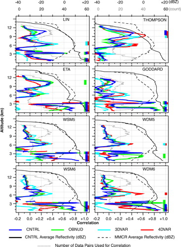
Fig. 8 Average contributions (%) of individual hydrometeor species (colours, coded at top) to total simulated cloud radar reflectivity for eight WRF microphysics schemes for CNTRL and data assimilation (DA) experiments (OBNUD, 3DVAR, 4DVAR) at five representative altitudes (1, 3, 5, 7, 9 km) for 27–31 May 2001. The overall contributions were computed by averaging hydrometeor reflectivity contributions (e.g. see Fig. 6 for CNTRL) over the simulation period. Simulated cloud radar reflectivity was computed using particle size distribution (PSD) characteristics for individual microphysics schemes (Table 1) and averaged over the 9×9 grid points nearest to the SGP CF (Fig. 1, dark dotted square). For Eta microphysics, snow and ice are not differentiated. WRF single/double-moment five-category scheme (WSM5/WDM5) provides explicit treatment of cloud water, rainwater, snow and ice species. Lin, WSM6, WDM6, Goddard and Thompson microphysics schemes predict the additional graupel species.

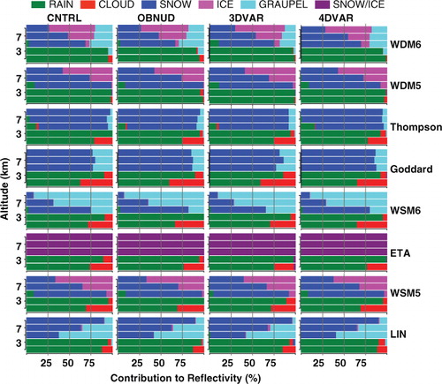
Fig. 9 Frequency bias scores (FBSs) (Section 2.3) as a function of reflectivity threshold from − 35 to + 15 dBZ at 1 dBZ intervals for eight WRF microphysics scheme simulations with (colours, defined at top) and without (CNTRL, dark lines) data assimilation (DA). Cloud radar reflectivity values were averaged over the 9×9 grid points nearest to the SGP CF (Fig. 1, dark dotted square). FBS values shown are limited to a maximum of 1.5 because of their steep increases for reflectivity thresholds exceeding + 15 dBZ. Grey-shaded envelope contains the 95% bootstrap confidence intervals (CIs) (Section 2.3) for CNTRL FBSs. Thick broken dark horizontal lines show FBS values for perfect model skill. OBNUD is surface and rawinsonde observation nudging and 3DVAR and 4DVAR are three-dimensional and four-dimensional variational DA, respectively.

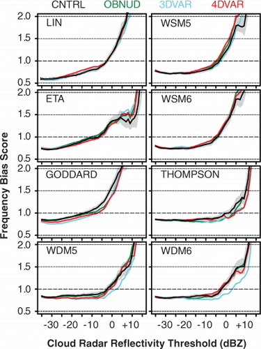
Fig. 10 Same as Fig. 9, but for equitable threat scores (ETSs) for cloud radar reflectivity thresholds between − 35 to + 15 dBZ at 1 dBZ intervals.

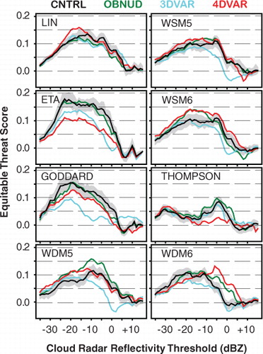
Fig. 11 Simulated water vapour and observed cloud reflectivity information for convective event A (2300 UTC 27 May–0100 UTC 28 May, 2001). Left panels enclose inner-nested model domain (Fig. 1) within which coloured straight lines (coded at top right) locate across-storm-line axes for eight CNTRL [without data assimilation (DA)] microphysics simulations, constructed as described in Section 4.3. Contours in left panels give simulated mixing ratio distribution (g kg⁻¹) for a representative microphysics scheme (Lin, top left) and selected large mixing ratios for all eight CNTRL microphysics schemes (bottom left, colour coded at top right) at level of maximum observed CF MMCR reflectivity (5.5 km AGL). Crosses in left panels locate CF. Right panels present hourly sequence of WSR-88D Level III reflectivity fields (lowest elevation angle) from Vance AFB radar (Fig. 1), and the locations of the inner-nested model domain and its simulated across-storm-line axes, above. Black arrows in top two right panels identify the line storm investigated.

Fig. 12 Vertical structure of observed convection characteristics in the vicinity of the CF for 2100 UTC 27 May–0700 UTC 28 May 2001. (a) Time–height section of MMCR-observed raw reflectivity (with clutter removed, colour scale at bottom right), showing complete attenuation at time of maximum convection. (b) Same section for MMCR-observed reflectivity best estimate (Mace et al., 2006, colour scale at bottom right) and equivalent potential temperature from CF rawinsonde (black contours, K). In (b), arrows at top indicate times of data used for simulation result averaging in Figs. (13–16), and thick black dashed line is the 0°C isotherm. (c) Rawinsonde-based saturated moist static energy deviations (, contours, K) and buoyancy perturbations (B, shading, scale at bottom right) for the lowest 3 km. (d) Skew T–log p diagram comparing CF rawinsonde observations (blue and grey curves) and a representative CNTRL simulation (Lin microphysics, red curves) averaged over the 9×9 grid points nearest to the CF (Fig. 1, dark dotted square) for 0000 UTC 28 May 2001. Red broken line in (d) indicates surface-500 m layer CAPE. Rawinsonde launch times nearest to and within 2100 UTC 27 May–0700 UTC 28 May period were 2030, 2330, 0530 UTC. Parts of the extended low-level MMCR radar echoes below 3 km in (b) likely are contaminated by radar signals from non-cloud sources.

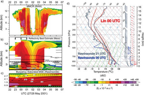
Fig. 13 Vertical structure of simulated convection characteristics along axes in Fig. 11 for eight CNTRL (without data assimilation [DA]) microphysics simulations averaged over 3-hourly time-steps centred on 0000 UTC 28 May 2001. Top and third rows contain horizontal-height cross-sections of Ka-band cloud radar reflectivity (shading, dBZ, colour coded at bottom) and equivalent potential temperature (contours, K), where thin black broken lines are 0°C isotherms. Second and fourth rows have same sections for lowest 3 km for perturbations of moist static energy (, contours, K) and buoyancy (B, shading, colour coded at bottom), computed as described in Section 4.3. For each microphysics scheme, all variables were averaged over 27 km normal to its axis in Fig. 11 (see Section 4.3). Thick horizontal red lines between panels indicate west-to-east extent of the Central Facility (CF) vicinity enclosed by dark dotted square in Fig. 1. The CF location is indicated by red arrows at bottom.

Fig. 14 Comparison of CNTRL (without data assimilation [DA]) WRF-ARW microphysics-simulated versus MMCR/rawinsonde-observed vertical profiles of cloud and atmospheric properties in CF vicinity for 2300 UTC 27 May–0600 UTC 28 May 2001. MMCR (rawinsonde) observations are instantaneous 0000 (0000 and 0600) UTC measurements at CF. All simulated values are 3-hourly averages (2300, 0000, 0100 UTC) for 9×9 grid points surrounding CF (Fig. 1). (a) MMCR-observed (red line) and simulated (other colours, coded at top) Ka-band cloud radar reflectivity. (b)–(e) Relative humidity (RH), CAPE, CIN and equivalent potential temperature (θ _e) from rawinsonde observations (red, solid is 0000 UTC, broken is 0600 UTC) and simulations (other colours, coded at top). (f)–(h) Buoyancy (B), perturbation equivalent potential temperature () and perturbation saturated moist static energy () relative to time-averaged reference profiles (see Section 4.3) for rawinsonde observations (red, solid is 0000 UTC, broken is for 0600 UTC) and simulations (other colours, coded at top). Blue lines in (f)–(h) are corresponding perturbation values, but averaged for all eight microphysics simulations and computed relative to area-averaged (35×35 grid points, Fig. 1) reference profiles (see Section 4.3). Grey envelopes in (b)–(h) span the 95% two-sided confidence intervals (CIs) (t-interval; Tamhane and Dunlop, 2000, pp. 249–250) for the average of the eight microphysics CNTRL values.

Fig. 15 Same as Fig. 13 except for 4DVAR simulations. The cross-sections for each microphysics simulation are constructed along the same horizontal axis as was obtained and used for the corresponding CNTRL (without data assimilation [DA]) simulation (Fig. 11). See Section 4.3 for further explanation and justification.

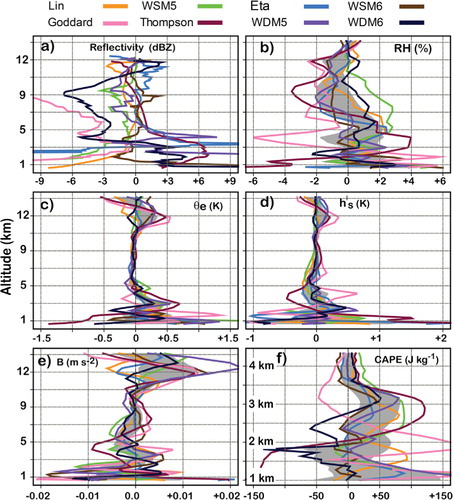
Fig. 16 Comparison of 4DVAR microphysics-simulated vertical profiles of cloud and atmospheric properties in CF vicinity with counterpart CNTRL simulations (Fig. 14) for 2300 UTC 27 May–0100 UTC 28 May 2001. All simulated values are 3-hourly averages (2300, 0000, 0100 UTC) for 9×9 grid points surrounding CF (Fig. 1). 4DVAR-minus-CNTRL simulation differences (microphysics scheme colour coded at top) of (a) K_a-band cloud radar reflectivity (dBZ differences), (b) relative humidity (RH), (c) equivalent potential temperature (θ _e), (d) perturbation saturated moist static energy (), (e) buoyancy (B) and (f) CAPE. Perturbations (, B) are from time-averaged simulation reference profiles as described in Section 4.3. Grey envelopes in (b)–(f) span the 95% two-sided confidence intervals (CIs) (t-interval; Tamhane and Dunlop, 2000, pp. 249–250) for the average of the eight microphysics 4DVAR-minus-CNTRL values.

Rutledge S. A. , Hobbs P. V . The mesoscale and microscale structure and organization of clouds and precipitation in midlatitude cyclones. Part VIII: a model for the “seeder-feeder” process in warm-frontal rainbands. J. Atmos. Sci. 1983; 40: 1185–1206.

 Web of Science ®Google Scholar

Hong S.-Y. , Dudhia J. , Chen S.-H . A revised approach to ice microphysical processes for the bulk parameterization of clouds and precipitation. Mon. Wea. Rev. 2004; 132: 103–119.

 Web of Science ®Google Scholar

Houze R. A. Jr , Hobbs P. V. , Herzegh P. H. , Parsons D. B . Size distributions of precipitation particles in frontal clouds. J. Atmos. Sci. 1979; 36: 156–162.

 Web of Science ®Google Scholar

Thompson G. , Field P. R. , Rasmussen R. M. , Hall W. D . Explicit forecasts of winter precipitation using an improved bulk microphysics scheme. Part II: implementation of a new snow parameterization. Mon. Wea. Rev. 2008; 136: 5095–5115.

 Web of Science ®Google Scholar

Morrison H. , Thompson G. , Tatarskii V . Impact of cloud microphysics on the development of trailing stratiform precipitation in a simulated squall line: comparison of one- and two-moment schemes. Mon. Wea. Rev. 2009; 137: 991–1007.

 Web of Science ®Google Scholar

Field P. R. , Hogan R. J. , Brown P. R. A. , Illingworth A. J. , Choularton T. W. , co-authors . Parameterization of ice-particle size distributions for mid-latitude stratiform cloud. Q. J. Roy. Meteorol. Soc. 2005; 131: 1997–2017.

 Web of Science ®Google Scholar

Lim K.-S. S. , Hong S.-Y . Development of an effective double-moment cloud microphysics scheme with prognostic cloud condensation nuclei (CCN) for weather and climate models. Mon. Wea. Rev. 2010; 138: 1587–1612.

 Web of Science ®Google Scholar

Mace G. G. , Benson S. , Sonntag K. L. , Kato S. , Min Q. , co-authors . Cloud radiative forcing at the atmospheric radiation measurement program climate research facility: 1. Technique, validation, and comparison to satellite-derived diagnostic quantities. J. Geophys. Res. 2006; 111 D11S90.

 Web of Science ®Google Scholar

Tamhane A. C. , Dunlop D. D . Statistics and Data Analysis: From Elementary to Intermediate.

 Google Scholar

Ferrier B. S. , Jin Y. , Lin Y. , Black T. , Rogers E. , co-authors . Implementation of a new grid-scale cloud and rainfall scheme in the NCEP Eta model. Preprints. 15th Conference on Numerical Weather Prediction. 2002; Boston: American Meteorological Society. 280–283.

 Google Scholar

Gallus W. A. Jr , Bresch J. F . Comparison of impacts of WRF dynamic core, physics package, and initial conditions on warm season rainfall forecasts. Mon. Wea. Rev. 2006; 134: 2632–2641.

 Web of Science ®Google Scholar