Figures & data
Fig. 1 Results of EnKF on a Lorenz96 data set (see Section 4) with 400 different combinations of diagonal and
matrices. RMSE was computed by comparing the filter output to the time series without observation noise. The correct Q and R (used to generate the simulated data) were diagonal matrices with entries
and
, respectively. The RMSE of the signal prior to filtering was 0.44 (shown as red dotted line) the RMSE of the optimal filter using
and
was 0.20 (shown as black dotted line). In (a) we show the effect of varying
when
and in (b) the effect of varying
when
.
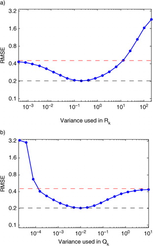
Fig. 2 We show the long-term performance of the adaptive EnKF by simulating Lorenz96 for 300 000 steps and running the adaptive EnKF with stationarity . (a) First row, left to right: true Q matrix used in the Lorenz96 simulation, the initial guess for
provided to the adaptive filter, the final
estimated by the adaptive filter, and the final matrix difference
. The second row shows the corresponding matrices for R; (b) RMSE of
as
is estimated by the filter; (c) RMSE of
as
is estimated by the filter; (d) comparison of windowed RMSE vs. number of filter steps for the conventional EnKF run with the true Q and R (black, lower trace), and the conventional EnKF run with the initial guess matrices (red, upper trace), and our adaptive EnKF initialised with the guess matrices (blue, middle trace).
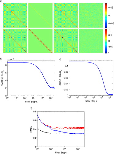
Fig. 3 A Lorenz96 data set with slowly varying Q is produced by defining the system noise covariance matrix Qk
as a multiple of the identity matrix, with the multiple changing in time. (a) Trace of Qk
(black) and for the EnKF (red) compared to the trace of
(normalised by N=40) for the Adaptive EnKF at stationarity levels
(green) and
(blue). (b) Comparison of the RMSE in state estimation for the EnKF with fixed
(red) and the Adaptive EnKF with stationarity
(green) and
(blue). The black curve represents an oracle EnKF which is given the correct covariance matrix Q at each point in time.
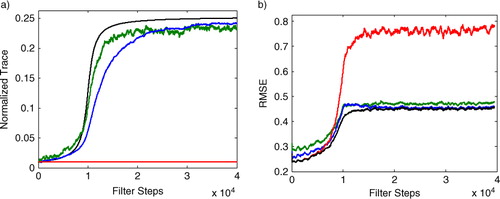
Fig. 4 We apply the adaptive EnKF with a sparse observation by only observing every other site (20 total observed sites) of a Lorenz96 simulation with 100000 steps. The matrix is assumed to be constant on 4×4 sub-matrices and the true Q used in the simulation is given the same block structure. (a) First row, left to right: true Q matrix used in the Lorenz96 simulation, the initial guess for
provided to the adaptive filter, the final
estimated by the adaptive filter, and the final matrix difference
. The second row shows the corresponding matrices for R; (b) RMSE of
as
is estimated by the filter; (c) RMSE of
as
is estimated by the filter; (d) comparison of windowed RMSE vs. number of filter steps for the conventional EnKF run with the true Q and R (black, lower trace), and the conventional EnKF run with the initial guess matrices (red, upper trace), and our adaptive EnKF initialised with the guess matrices (blue, middle trace).
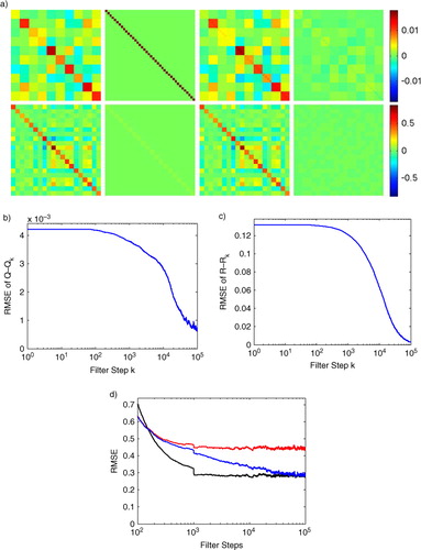
Fig. 5 We illustrate the effect of extremely sparse observations by only observing every fourth site (10 total observed sites) of the Lorenz96 simulation, the matrix is assumed to be constant on 4×4 sub-matrices and the true Q used in the simulation is given the same block structure. (a) First row, left to right: true Q matrix used in the Lorenz96 simulation, the initial guess for
provided to the adaptive filter, the final
estimated by the adaptive filter, and the final matrix difference
. The second row shows the corresponding matrices for R; (b) RMSE of
as the adaptive EnKF is run; (c) comparison of windowed RMSE vs. number of filter steps for the conventional EnKF run with the true Q and R (black, lower trace), and the conventional EnKF run with the initial guess matrices (red, upper trace), and our adaptive EnKF initialised with the guess matrices (blue, middle trace); (d) Enlarged view showing filter divergence, taken from (c). Note that the conventional EnKF occasionally diverges even when provided the true Q and R matrices. The
found by the adaptive filter is automatically inflated relative to the true Q which improves filter stability as shown in (c) and (d).
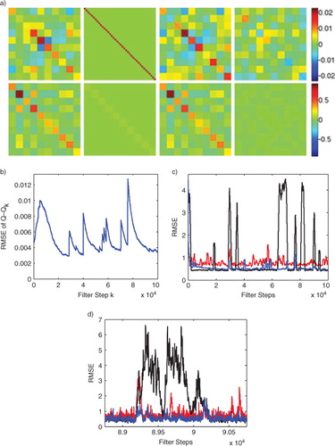
Fig. 6 For the first 10000 filter steps the model is correct and then the underlying parameters are randomly perturbed at each site. The conventional EnKF is run with the initial true covariances and
; the adaptive EnKF starts with the same values but it automatically increases the system noise level (
) to compensate for the model error resulting in improved RMSE. (a) First row, left to right: true Q matrix used in the Lorenz96 simulation, the initial guess for
provided to the adaptive filter, the final
estimated by the adaptive filter, and the final matrix difference
. The second row shows the corresponding matrices for R; (b) Model error (black, dotted curve) measured as the percent change in the parameter F i at each site compared to the relative change in the corresponding diagonal entries of
found with the adaptive EnKF (blue, solid curve), diagonal (green, solid curve). (c) Results of the adaptive EnKF (blue) compared to conventional EnKF (red) on a Lorenz96 data set in the presence of model error. The green curve is an adaptive EnKF, where
is forced to be diagonal and the black curve shows the RMSE of an oracle EnKF which is provided with the true underlying parameters F i for both halves of the simulation.
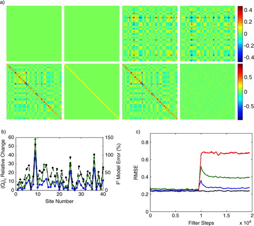
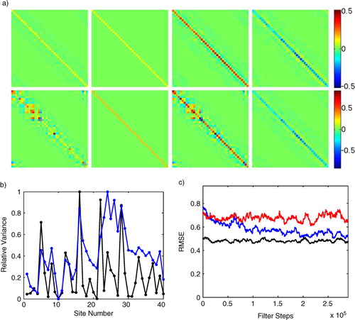
Fig. 7 We compare the conventional and adaptive LETKF on a simulation of 300000 steps of Lorenz96 (a) First row, left to right: benchmark matrix where Q is was the matrix used in the Lorenz96 simulation, the initial guess for
provided to the adaptive filter, the final
estimated by the adaptive filter, and the final matrix difference
. The second row shows the corresponding matrices for R (leftmost is the true R); (b) the variances from the diagonal entries of the true Q matrix (black, rescaled to range from 0 to 1) and the those from the final global estimate
produced by the adaptive LETKF (blue, rescaled to range from 0 to 1) (c) Results of the adaptive LETKF (blue) compared to conventional LETKF with the diagonal covariance matrices (red) and the conventional LETKF with the benchmark covariances
=
and
(black).