The role of model and initial condition error in numerical weather forecasting investigated with an observing system simulation experiment

Figures & data

Table 1. Description of all OSSE experiments included in this article

NR	Added Obs Err	Obs Network
Control	ECMWF	Yes	Operational 2005
NE	ECMWF	No	Operational 2005
DENSE	ECMWF	No	RAOBs
Twin Ctl	GEOS-5	Yes	Operational 2011
Twin NE	GEOS-5	No	Operational 2011

NR options are the ECMWF-generated NR or the identical twin GEOS-5 NR. ‘Added Obs Err’ refers to whether or not synthetic observation error was explicitly applied to synthetic observations. ‘Obs Network’ refers to the choice of synthetic observation network, with ‘operational’ the data types used operationally, and ‘RAOBs’ a hypothetical global network of rawinsondes only.

Fig. 1 Global analysis root-mean-square error (RMSE) for July. Left column, 30N–90N; centre column, 30S–90S; right column, 30S–30N. Top row, temperature (K); centre row, zonal wind (m s⁻¹); bottom row, specific humidity (kg kg⁻¹). Solid heavy line, NE experiment; heavy dashed line, Control experiment; heavy dash–dot line, DENSE experiment; thin solid line, Twin NE experiment; thin dashed line, Twin Control experiment.

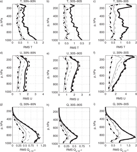
Fig. 2 Monthly mean analysis error on select model surfaces for the experiments in July, longitude on x-axis and latitude on y-axis. Left column, temperature at 500 hPa, K. Right column, zonal wind at 250 hPa, m s⁻¹. Note varying contour intervals between panels.

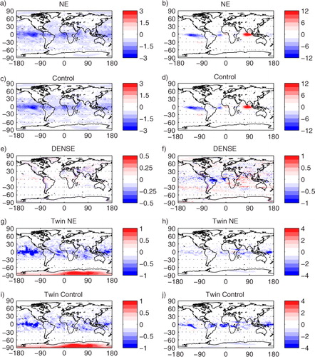
Fig. 3 Zonal mean time mean analysis increment (left column) and MAER (right column) for temperature (K), July, η-level pressure on y-axis and latitude on x-axis. Negative values of MAER indicate an improvement of the analysis field compared to the background. Note different contour range for Twin and ECMWF NR experiments.

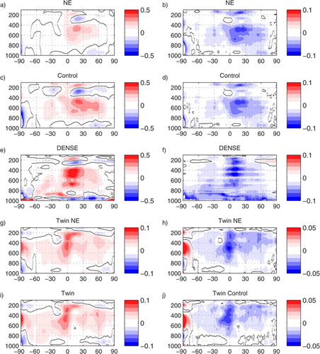
Fig. 4 Zonal mean time mean analysis increment (left column) and MAER (right column) for zonal wind (m s⁻¹), July, η-level pressure on y-axis and latitude on x-axis. Negative values of MAER indicate an improvement of the analysis field compared to the background. Note different contour range for Twin and ECMWF NR experiments.

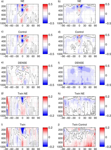
Fig. 5 Zonal mean variance in time of the analysis increment for temperature (K²), left, and zonal wind (m² s⁻²), July mean.

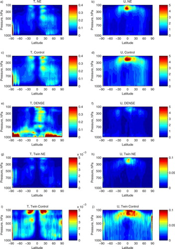
Fig. 6 Forecast root-mean-square error (RMSE) for temperature, July mean. Left column, 30N–90N; centre column, 30S–90S; right column, 30S–30N. Top row, 24 hour forecast; bottom row, 120 hour forecast. Solid heavy line, NE experiment; heavy dashed line, control experiment; heavy dash–dot line, DENSE experiment; thin solid line, Twin NE experiment; thin dashed line, Twin Control experiment.

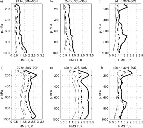
Fig. 7 As for Fig. 6, but for zonal wind u, m s⁻¹.

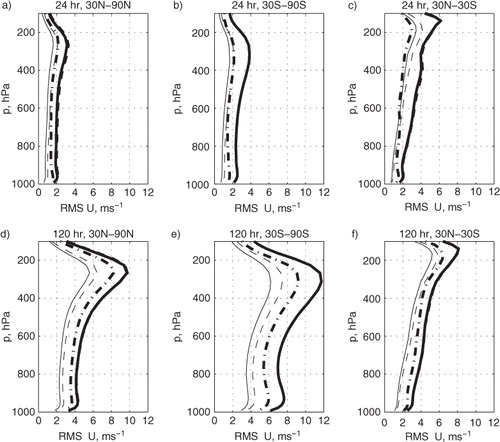
Fig. 8 Global error variance as a function of forecast time, July mean. Left column, 500 hPa temperature (K²); right column, 250 hPa zonal wind (m² s⁻²). Top row, 30N–90N; centre row, 30S–90S; bottom row, 30N–30S. Solid heavy line, NE experiment; heavy dashed line, control experiment; heavy dash–dot line, DENSE experiment; thin solid line, Twin NE experiment; thin dashed line, twin control experiment.

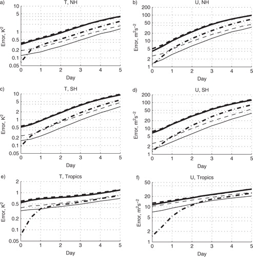
Fig. 9 12-Hour forecast error variance minus the analysis error variance for the month of July. Left column, temperature variance (contour interval 0.1 K²) on model surface nearest 500 hPa; right column, zonal wind variance (contour interval 1.5 m² s⁻²) on model surface nearest 250 hPa. x-axis, longitude; y-axis, latitude. Top, DENSE experiment; centre, Control experiment; bottom, Twin Control experiment.

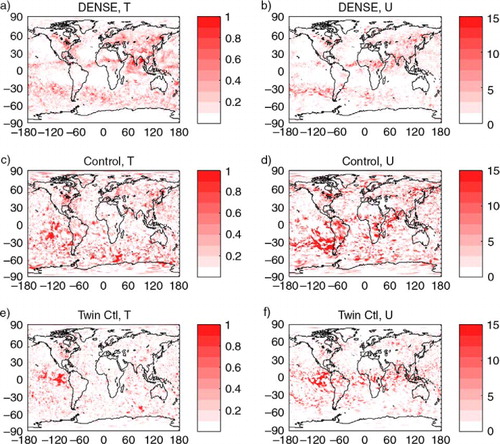
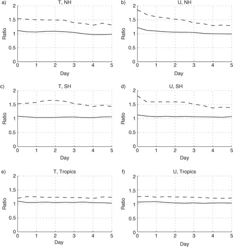
Table 2. Doubling times in days for RMSE of temperature and zonal wind, calculated using a fit to forecast error from 48 to 96 hours

Temperature			Zonal Wind
NH	SH	Tropics	NH	SH	Tropics
Control	2.8	2.3	10.7	2.6	2.6	7.7
NE	2.5	2.3	10.7	2.4	2.6	6.9
DENSE	2.5	2.0	7.7	2.2	2.0	4.8
Twin Ctl	2.8	2.3	9.2	2.5	2.3	7.7
Twin NE	2.5	2.0	8.2	2.2	2.1	6.9

Fig. 10 Ratio of areal mean error variances as a function of forecast time between the Control and NE experiments (solid line) and between the Twin Control and Twin NE experiments (dashed line), July. Top row, 30N–90N; centre row, 30S–90S; bottom row, 30N–30S. Left column, ratio for temperature at 500 hPa; right column, ratio for zonal wind at 250 hPa.