Figures & data
Fig. 1 Example OSTIA SST field for 1 July 2013 showing (a) global land/sea/lake mask with (b–d) close-ups of regions for detail. Colourbar in K.
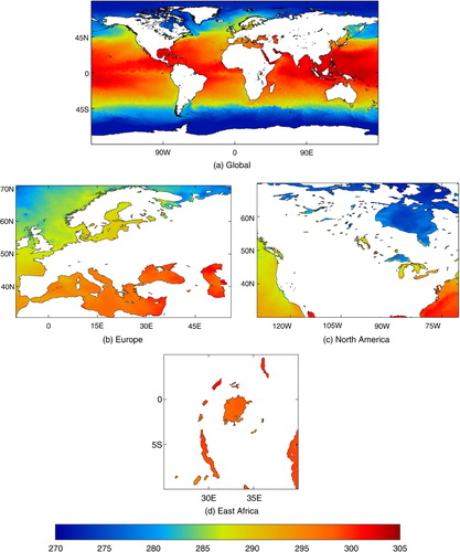
Table 1. Accuracy of operational SST algorithms when used for LSWT
Table 2. Accuracy of LSWT algorithms designed for lakes
Fig. 2 Total daily number of observations by instrument type for all lakes in OSTIA mask, for JJA 2009.
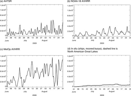
Table 3. Observation-minus-background statistics for JJA 2009, for all lakes in global OSTIA mask and three case studies
Table 4. OSTIA LSWT minus ARC-Lake observations and ARC-Lake climatology minus ARC-Lake observations for JJA 2009 for selected lakes, listed in order of descending surface area
Fig. 3 OSTIA LSWT analysis minus ARC-Lake observations for each lake, for JJA 2009, with absolute latitude (i.e. disregarding hemisphere) with (a) RMS and (b) mean difference. Each point represents a lake. A red triangle indicates the lake has an elevation over 2500 m, and a black dot equal to or below 2500 m. A blue square indicates the lake also has a surface area of greater than 3000 km2.
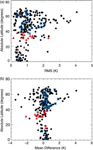
Fig. 4 OSTIA LSWT minus ARC-Lake observations for each lake, for JJA 2009, with isoperimetric quotient (a measure of how close to circular the lake is, or the regularity of the coastline, see text) with (a) RMS and (b) mean difference.
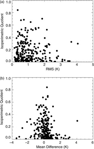
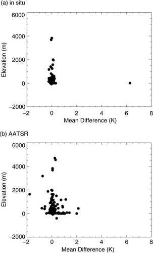
Fig. 5 Mean difference of (a) in situ observations minus OSTIA LSWT background and (b) AATSR observations minus OSTIA LSWT background. For each lake with available observations, for JJA 2009, with elevation. Note that 83% of in situ observations are located in the North American Great Lakes, whereas AATSR is spread globally.