Hybrid algorithm of ensemble transform and importance sampling for assimilation of non-Gaussian observations

Figures & data

Fig. 1 Outline of the hybrid approach proposed in the present paper.

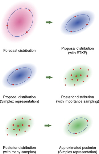
Table 1. Results of experiments with the linear Gaussian observation model

RMSE (σ=0.5)		RMSE (σ=1.0)
Hybrid filter	ETKF	Hybrid filter	ETKF
N=16	0.84	0.62	4.31	3.44
N=18	0.18	0.19	0.71	0.50
N=20	0.18	0.19	0.39	0.41
N=24	0.19	0.20	0.39	0.41
N=28	0.19	0.20	0.40	0.42
N=32	0.19	0.20	0.40	0.43
N=36	0.19	0.21	0.40	0.43

Table 2. Results of experiments with the nonlinear Gaussian observation model

RMSE (σ=0.5)		RMSE (σ=1.0)
Hybrid filter	ETKF	Hybrid filter	ETKF
N=16	1.36	2.24	5.15	4.93
N=18	0.19	0.20	4.79	4.69
N=20	0.19	0.20	2.96	3.89
N=24	0.19	0.21	1.33	1.12
N=28	0.19	0.21	0.89	0.79
N=32	0.20	0.21	0.43	0.68
N=36	0.20	0.22	0.43	0.59

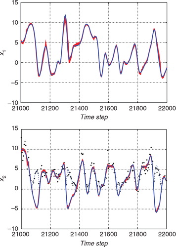
Fig. 2 Result of the estimation from the nonlinear observation with the standard ETKF algorithm. The upper panel shows the estimate for x ₁ (an unobserved variable) and the lower panel shows the estimate for x ₂ (an observed variable). The blue line indicates the true state. The red line indicates the estimate. The thin red dashed lines indicate the 2σ range of the filtered distribution.

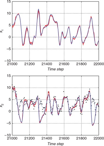
Fig. 3 Result of the estimation from the nonlinear observation with the hybrid algorithm. As in Fig. 2, the upper and lower panels show the estimates for x ₁ (an unobserved variable) and the estimate for x ₂ (an observed variable), respectively. The blue line indicates the true state and the red line indicates the estimate. The thin red dashed lines indicate the 2σ range of the filtered distribution.

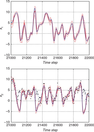
Fig. 4 The standard deviations of the forecast distribution (green line), the proposal distribution (blue line), and the filtered distribution (red line) for the estimation from the nonlinear observation with the hybrid algorithm. The upper and lower panels show the standard deviations for x ₁ (an unobserved variable) and those for x ₂ (an observed variable), respectively.

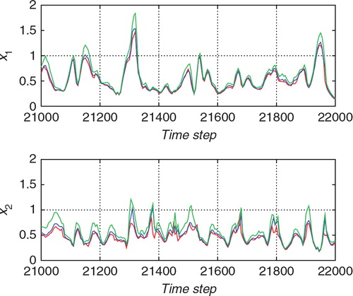
Fig. 5 The number of particles used for the Monte Carlo step J for the estimation from the nonlinear observation with the hybrid algorithm.

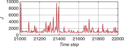
Fig. 6 The ratio between the effective sample size J _eff and J for the estimation from the nonlinear observation with the hybrid algorithm.

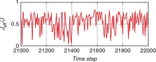
Fig. 7 Superposition of 50 trials of the estimates from the nonlinear observation with the standard ETKF algorithm (red lines) and the true state (blue line). The upper and lower panels show the estimates for x ₁ (an unobserved variable) and the estimate for x ₂ (an observed variable), respectively.

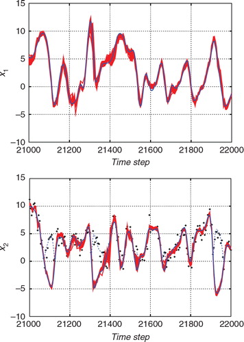
Fig. 8 Superposition of 50 trials of the estimates from the nonlinear observation with the hybrid algorithm (red lines) and the true state (blue line). The upper and lower panels show the estimates for x ₁ (an unobserved variable) and the estimate for x ₂ (an observed variable), respectively.

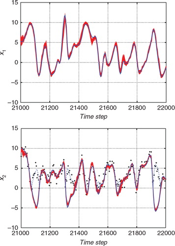
Fig. 9 Comparison between the root-mean-square of the deviation from the truth (red) and the ratio of the effective sample size J _eff to the total size J (blue) in the early stage of data assimilation.

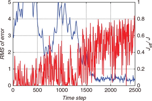
Table 3. Results of experiments with the non-Gaussian observation model

RMSE (σ=0.2)		RMSE (σ=0.4)
Hybrid filter	ETKF	Hybrid filter	ETKF
N=16	1.60	2.90	4.90	4.79
N=18	0.12	1.50	4.77	4.63
N=20	0.12	0.20	2.35	3.58
N=24	0.13	0.21	0.91	1.32
N=28	0.13	0.21	0.44	0.89
N=32	0.13	0.21	0.28	0.81
N=36	0.13	0.21	0.28	0.71

Fig. 10 Result of the estimation from the non-Gaussian observation with the standard ETKF algorithm. The upper and lower panels show the estimates for x ₁ (an unobserved variable) and the estimate for x ₂ (an observed variable), respectively. The blue line indicates the true state and the red line indicates the estimate. The thin red dashed lines indicate the 2σ range of the filtered distribution.

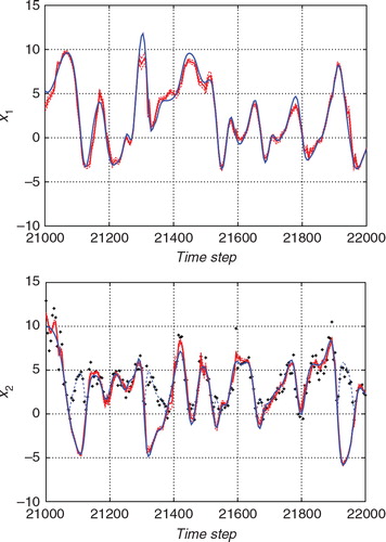
Fig. 11 Result of the estimation from the non-Gaussian observation with the hybrid algorithm. The upper and lower panels show the estimates for x ₁ (an unobserved variable) and the estimate for x ₂ (an observed variable), respectively. The blue line indicates the true state and the red line indicates the estimate. The thin red dashed lines indicate the 2σ range of the filtered distribution.

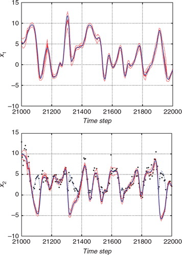
Fig. 12 Histogram of marginal of the filtered distribution of x ₂ at time step 21600 (t=216.00) for the case with the non-Gaussian observation. The estimate using the ETKF (blue line), the true state (solid vertical line), and the observed value (dashed vertical line) are also shown.

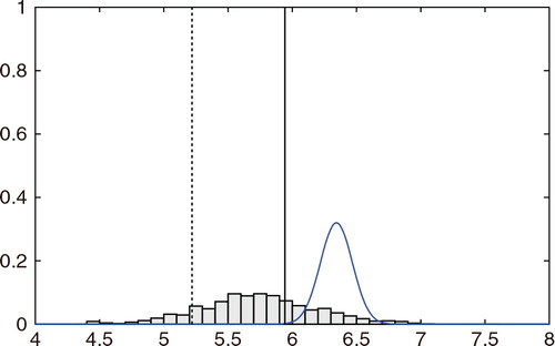
Fig. 13 The standard deviations of the forecast distribution (green line), the proposal distribution (blue line), and the filtered distribution (red line) for the estimation from the non-Gaussian observation with the hybrid algorithm. The upper and lower panels show the standard deviations for x ₁ (an unobserved variable) and those for x ₂ (an observed variable), respectively.

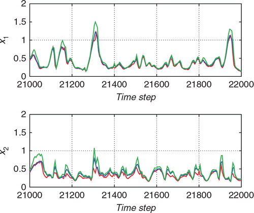
Fig. 14 The number of particles used for the Monte Carlo step J for the estimation from the non-Gaussian observation with the hybrid algorithm.

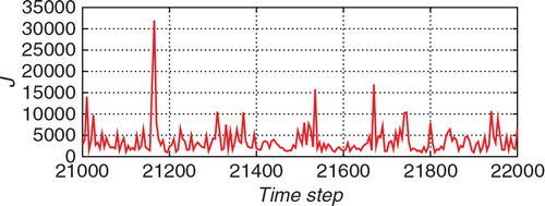
Fig. 15 The ratio between the effective sample size J _eff and J for the estimation from the non-Gaussian observation with the hybrid algorithm.

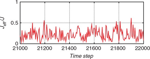
Fig. 16 Superposition of 50 trials of the estimates from the non-Gaussian observation with the standard ETKF algorithm (red lines) and the true state (blue line). The upper and lower panels show the estimates for x ₁ (an unobserved variable) and the estimate for x ₂ (an observed variable), respectively.

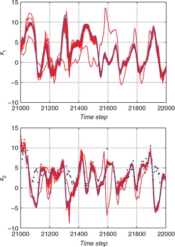
Fig. 17 Superposition of 50 trials of the estimates from the non-Gaussian observation with the hybrid algorithm (red lines) and the true state (blue line). The upper and lower panels show the estimates for x ₁ (an unobserved variable) and the estimate for x ₂ (an observed variable), respectively.