Mechanisms controlling the onset of simulated convectively coupled Kelvin waves

Figures & data

Fig. 1 Decomposition of precipitation as a function of wave phase (x/λ, where x is position and λ is the horizontal wavelength) in a simple model of RF07 for the eastward-moving convectively coupled Kelvin mode with zonal wavenumber l=5.5. The solid line is the total precipitation (left hand side of equation 4); the short dashed line (P ₁) is the contribution due to saturation fraction; the long dashed line (P _2t ) is the CIN contribution; and the dotted line (P _2s ) is the contribution due to surface fluxes.

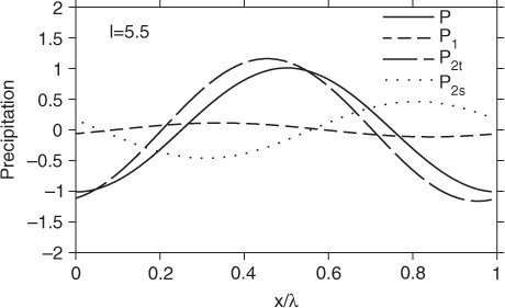
Fig. 2 The modelled evolution of rainfall over the 7000 km domain. The contour intervals are 20 mm day⁻¹, with a maximum values ranging between 60 and 100 mm day⁻¹. The wave speed is about 15 ms⁻¹ toward the east (right).

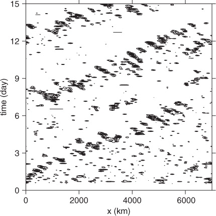
Fig. 3 Same as Fig. 2, but plotted in a reference frame moving at the phase speed of the wave (15 ms⁻¹). In this reference frame, the wave is initiated on the right side of the strip of precipitation (approximately 6000 km), and the decay is on the left edge (3500 km).

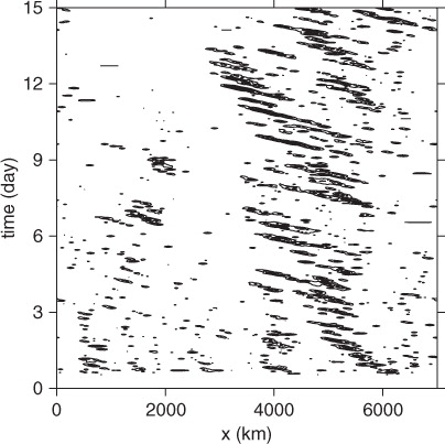
Fig. 4 Contours show the modelled mass flux for CCKW as a function of height. For comparison, the rain rate is shown with a solid line.

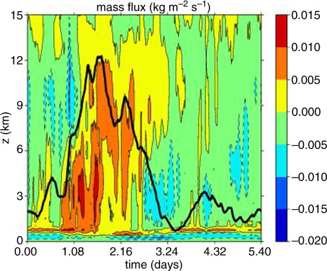
Fig. 5 The top panel shows the modelled precipitation rate for CCKW as a function of time; the middle panel shows modelled DCIN is solid line (dashed line is precipitation rate); and the bottom panel shows modelled threshold moist entropy, , and the boundary layer moist entropy, s _bl .

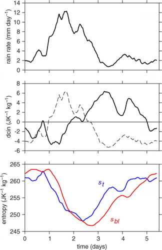
Fig. 6 Modelled saturated moist entropy anomalies are shown in contours; rain is shown with a solid line.

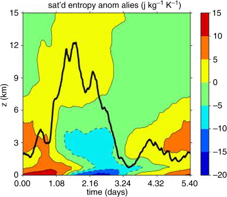
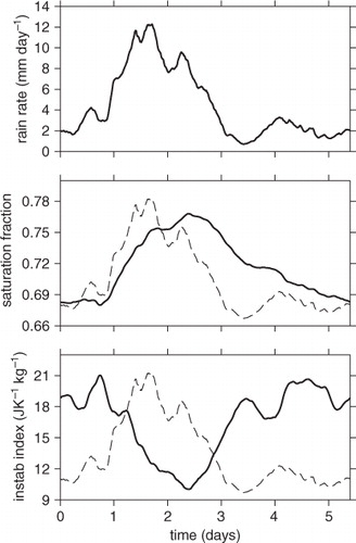
Fig. 7 The top panel shows the modelled precipitation rate for a CCKW as a function of time; the middle panel shows the modelled saturation fraction; and the bottom panel shows the modelled instability index.