Dual-Doppler radar analysis of a near-shore line-shaped convective system on 27 July 2011, Korea: a case study

Figures & data

Fig. 1 Observation sites of Doppler radar with geographical height. The open circle and quadrangle are the observation ranges of Doppler radar.

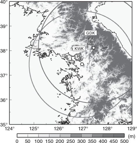
Fig. 2 The accumulated rainfall amount (mm) over the Korea during 3 hours (07–10 LST) and time series of temperature (°C, solid line), wind direction and speed (m s⁻¹, barb) and rainfall amount (mm hr⁻¹, bar graph) observed at Gwanak and Song-do AWS station on 27 July 2011. Half and full barbs are 5 and 2.5 m s⁻¹, respectively.

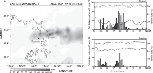
Fig. 3 Surface weather map at 0300 LST on 27 July 2011.

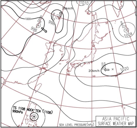
Fig. 4 MASAT-IR black-body brightness temperature (°C) distribution over the Korean peninsula at 0900 LST on 27 July 2011. Dashed white box (M1) indicates domain for radar analysis.

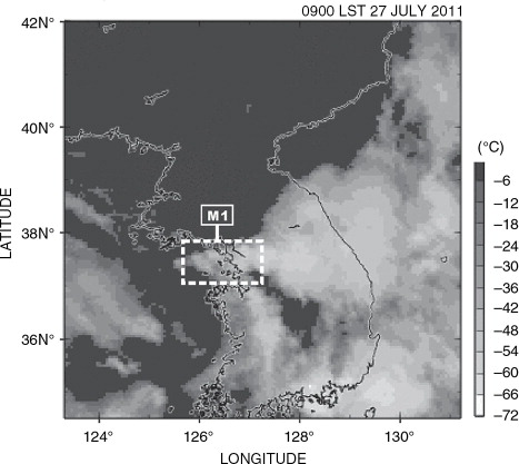
Fig. 5 Mesoscale analysis for 0600 LST, 27 July 2011: (a) equivalent potential temperature θ _e (K, shaded), geopotential height (gpm, contoured every 10 gpm) and horizontal wind vector and speed (m s⁻¹, barbs); (b) θ _e (K, shaded), temperature (°C, contour) and horizontal wind vector and speed (m s⁻¹, barbs).

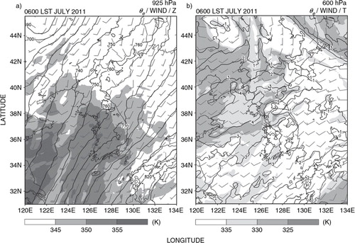
Fig. 6 Horizontal distribution of reflectivity at 2 km ASL for (a) 0700 LST, (b) 0720 LST, (c) 0740 LST, (d) 0800 LST, (e) 0820 LST, (f) 0840 LST, (g) 0900 LST, (h) 0920 LST, (i) 0940 LST and (j) 1000 LST on 27 July 2011. The contour interval of reflectivity is 5 dBZ from 35 dBZ and small open circles indicate the location of the radar station (KWK). The tee quadrilateral boxes (S1, S2 and S3) demark the regions used for the analysis of the precipitation system.

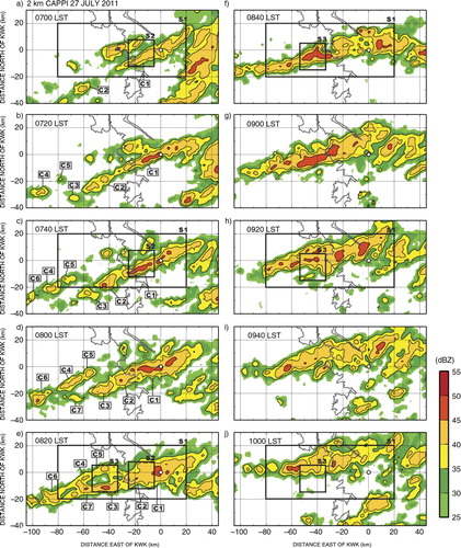
Fig. 7 Time series of the horizontal area of the convective region (reflectivity greater than 45 dBZ) at 2 km (solid line), 4 km (dotted line) and 6 km (dashed line) ASL in S1 analysis domain. The boundary of the analysis domain (S1) is shown in Fig. 6.

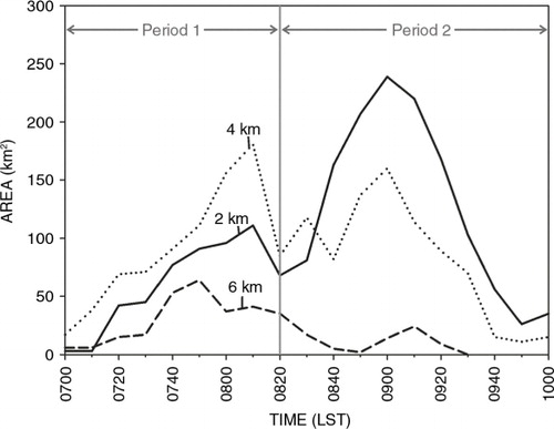
Fig. 8 Appearance rate distribution of radar reflectivity of precipitation system in an east-west direction with height. This appearance rate is averaged in a south-north direction as M1 analysis domain shown in Fig. 4b. (a) and (b) were averaged from 0700 LST to 0820 LST and 0830 LST to 0950 LST, respectively.

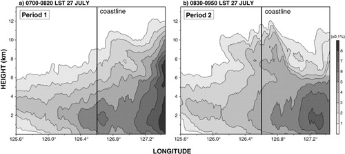
Fig. 9 Horizontal distributions of reflectivity, divergence and wind field in selected time (0750–0800 LST). A small open circle indicates the location of the radar station (KWK) and the thick grey contour line in each panel represents the coastline. The first column (a)–(b) shows the radar reflectivity at 2 km ASL. The contour interval of reflectivity is 5 dBZ from 35 dBZ and areas with reflectivity between 25 and 55 dBZ are shaded. The second column (c)–(d) shows the shaded divergence areas of 0.5 km ASL and contoured reflectivity like (a)–(b). The third column (e)–(f) shows the horizontal wind vectors and contoured reflectivity at 0.5 km ASL. The cross-section lines of (a) and (b) panels are presented in Fig. 10.

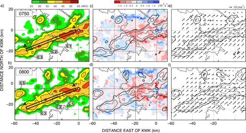
Fig. 10 The reflectivity, vertical velocity, divergence and wind fields of the vertical cross-sections averaged in the thin box (A–A’) as time of Fig. 9. The thick grey line on the horizontal axis indicates the coastline. The location of thin box is presented in each panel of Fig. 9a, b. The solid line and dashed line in (a)–(d) are positive and negative value of vertical velocity (m s⁻¹, every 0.3), respectively. Thin contours in (e)–(h) indicate radar reflectivity from 35 dBZ with contour interval of 5 dBZ and thick contours are convective region in excess of 45 dBZ. The grey lines on the horizontal axis indicates the coastline.

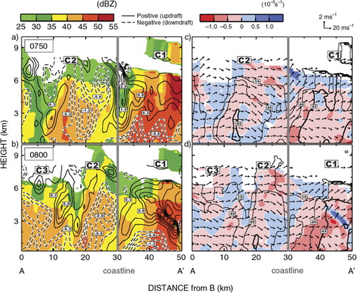
Fig. 11 Same as Fig. 9. The cross-section lines of (a) and (b) panels are presented in Fig. 12.

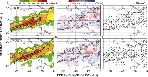
Fig. 12 Same as Fig. 10 except for lines B–B’ and C–C’ in Fig. 11a, b.

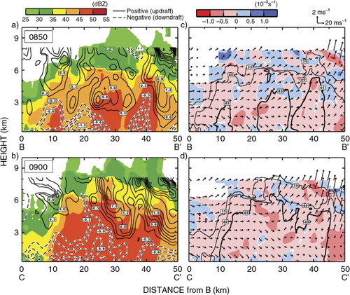
Fig. 13 Time–height cross-section of maximum reflectivity, vertical velocity and averaged divergence for each period in the analysis domains. (a), (c) and (e) are on the onshore (S2) and (b), (d) and (f) are on the offshore (S3). The boundaries of the analysis domains are depicted in Fig. 6.

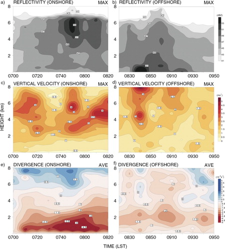
Fig. 14 Mean profiles of divergence in S2 (onshore) and S3 (offshore) analysis domain at selected times.

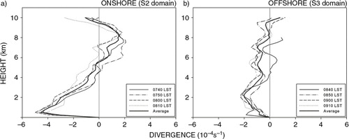
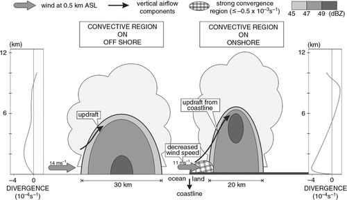
Fig. 15 Schematic representation of convective region in precipitation system at offshore and onshore. Shading region indicates variation in the reflectivity of radar. Thick arrows shaded grey colour and thin black arrows are horizontal wind at 0.5 km ASL and vertical airflow components, respectively.