Figures & data
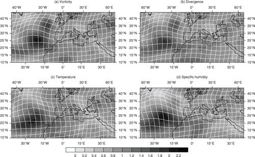
Fig. 1 Relative vorticity (shadings, s −1) in the ARPEGE analysis of the 7th of November 2011 (12UTC) at model level 60 (≈900 hPa). Also shown is the Geostrophic Transform, represented here as grid lines bending of a regular grid induced by the GT (solid black lines). The geographical contours are not represented for clarity but the domain is the same as in .
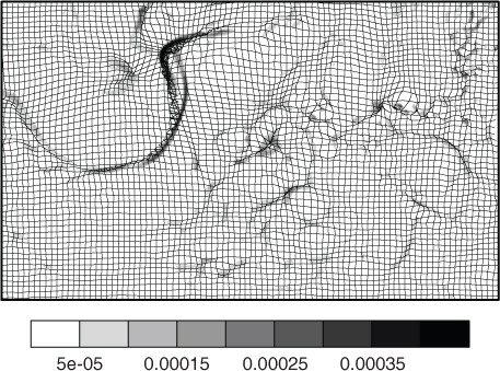
Fig. 2 Map of the meteorological situation of the 7th of November 2011 (12UTC) from the ARPEGE analysis. Vorticity (shadings, 10−4s−1) at model level 60 (≈900 hPa), sea surface pressure (dashed lines every 5 hPa) and winds at model level 35 (≈300 hPa) (only values over 60 kt, drawn in wind barbs). The large rectangle delimits the computational domain.
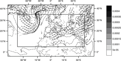
Fig. 3 Superposition of the correlation function (contoured at 0.4, 0.6, and 0.8 in dashed thin lines) with the ellipses determined from the inertia matrix (solid bold lines). Correlations are computed at level 60 (≈900 hPa) for (a) vorticity, (b) temperature, and (c) specific humidity. For divergence the superposition is very similar to the vorticity one but with smaller correlation lengths (not shown).
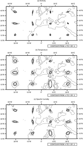
Fig. 4 Grid-lines bending of a regular grid induced by the deformation d. The resulting deformed grid represents in transformed space the contour of the physical space coordinate. Deformation presented in (a), (b), and (c) are objectively estimated with the ST. Different values of L are presented: (a) L=8 grid points, (b) L=12 grid points, and (c) L=20 grid points. Backgrounds of each panel represent values of det(J d ) the Jacobian determinant of the deformation at each grid point. Changing sign areas (noted with dashed thin lines) for det(J d) induced a crossing of deformed grid-lines causing non-invertibility. Those results are for the specific humidity at level 35 (≈300 hPa). (d) The corresponding grid-lines bending and the Jacobian determinant of the deformation estimated with the GT, with L=12 grid points.
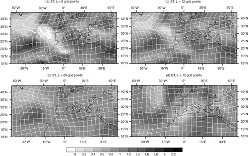
Fig. 5 Vertical profiles of the anisotropy O, for (a) vorticity, (b) divergence, (c) temperature, and (d) specific humidity, for the ensemble in physical space (solid lines) and in computational space after applying the inverse of the deformation estimated with the ST (dotted lines) and with the GT (dashed lines). O is averaged over the whole domain (except near boundary points) on the 7th of November 2011 at 12UTC.
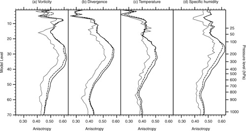
Fig. 6 Maps of anisotropy for (a) the raw ensemble, (b) the ensemble undeformed with the GT, and (c) the ensemble undeformed with the ST. The variable is temperature on the 7th of November 2011 at 12UTC at level 60 (≈900 hPa). Near boundaries points are also avoided. One notices that for the raw ensemble the background coast lines are exact. But for the two other panels, since the ensemble has been undeformed, they are not corresponding to the foreground and are just drawn to simplify the recognition of the features with the top panel.
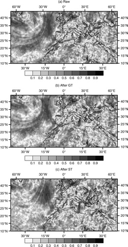
Fig. 7 Vertical profiles of the standard deviation of anisotropy O, for (a) vorticity, (b) divergence, (c) temperature, and (d) specific humidity, for the ensemble in physical space (solid lines) and in transformed space after applying the inverse of the deformation estimated with the ST (dotted lines), or after the GT (dashed lines). Results are averaged over the whole domain (except near boundary points) on the 7th of November 2011 at 12UTC for ARPEGE model.
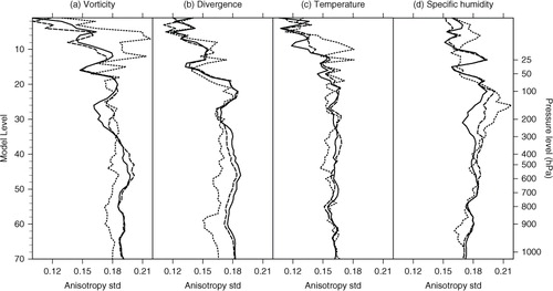
Fig. 8 Vertical profile of standard deviation of total length scale L t , for (a) vorticity, (b) divergence, (c) temperature, and (d) specific humidity, for the ensemble in physical space (solid line) and in transformed space after applying the inverse of the deformation estimated with the ST (dotted line), or after the GT (dashed line). Near boundary points were also neglected. Stratospheric model levels from 1 to 19 are not represented.
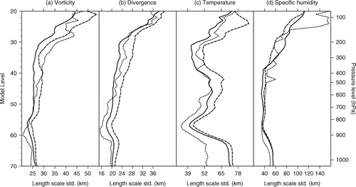
Fig. 9 Superposition of simplified elliptic visualisation of the correlation of the raw ensemble (solid lines) and of the ensemble in transformed space after ST (dashed lines). Correlation tensors are computed at level 60 (≈900 hPa) for temperature. For each position (4×5), ellipses for the raw ensemble and for the ensemble in transformed space are not superposed since error fields have been displaced by d −1.
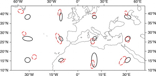
Fig. 10 Distribution histogram of anisotropy O over the domain for the raw ensemble (hatched bars, background) and the ensemble undeformed with the ST (filled bars, foreground), for specific humidity, on the 7th of November 2011 at 12UTC for ARPEGE model at the stratospheric level 25 (≈150 hPa).
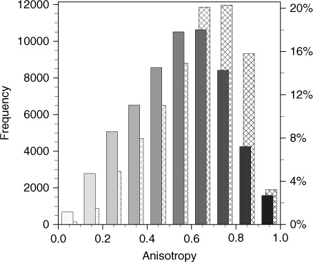
Fig. 11 Jacobian determinant of the deformation (grey shades) and the regular grid deformed by the deformation d (white lines, as ) estimated by ST for (a) vorticity, (b) divergence, (c) temperature, and (d) specific humidity, at level 60 (≈900 hPa).