
Figures & data
Fig. 1 (a) The cubed-sphere computational domain with Gauss–Lobatto–Legendre (GLL) points of N p ×N p in the N e elements, (b) zonally uniform flow over the isolated mountain at the initial time, (c) zonal wind field (contours, ms−1) after 14-day time integration.
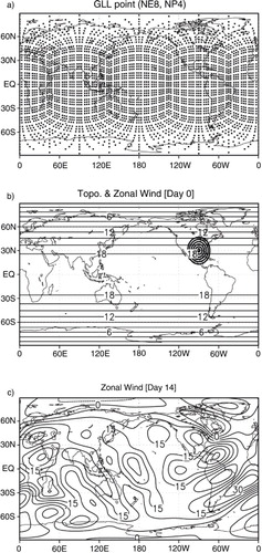
Fig. 2 Log of TL measures for (a) eq. (2a) and (b) eq. (2b) for each model state variable according to the scaling factor α. The vertical and horizontal axes are shown in logarithm scales.
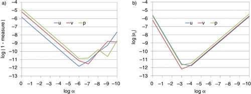
Fig. 3 Meridional wind fields after 15-day time evolution of the initial perturbation for (a) TLM and (b) difference of ‘perturbed’ and ‘unperturbed’ non-linear models. Contours are shown with 0.5 ms−1 intervals without the zero contours.
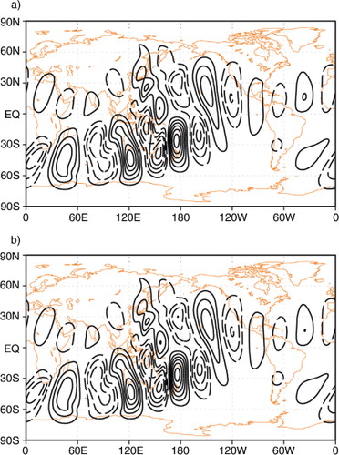
Fig. 4 Spreads of observational information with the colour shadings. (a) The structure of the initial sensitivity (time t=0) obtained by integrating ADM backwards in time and then by applying the covariance matrix P b in eq. (8). The zonal wind observation (×) is initially located at (35°W, 12.5°S) at 3 hour. Then, TLM is integrated with the initial sensitivity as the initial condition at time (b) 3, (c) 6, (d) 12, (e) 18 and (f) 24 hours, respectively. Arrows represent the wind vectors.
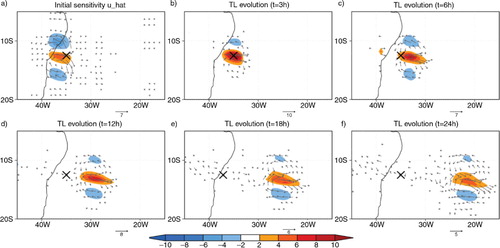
Fig. 5 Schematic flow of direct and indirect representer algorithms (middle column). The direct method in the left column first constructs the representer matrix explicitly by directly applying a series of models such as ADM, covariance and TLM, and then the linear equation in eq. (11) is solved for the representer coefficients β. The indirect method in the right column approximates the representer coefficients in eq. (11) by using iterative solvers.
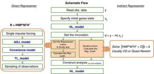
Fig. 6 Analysis increments for (a, b, c) zonal and (d, e, f) meridional wind fields in the single-observation experiments. EXP0 only uses variance information, while EXP2 and EXP4 used for a longer horizontal correlation. The observation location is denoted by the black ×. See Section 5.1 for more detail.
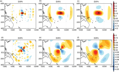
Fig. 7 Zonal wind fields (contours, ms−1) for the true state at 1, 2, 3, 4 and 5 hours from the initial condition. Black dots indicate selected observational locations.
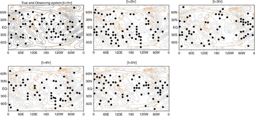
Fig. 8 Zonal wind fields (ms−1) for (a) guess and (b) the background error. The other panels (c–f) show the analysis increment for EXP0, EXP2 and EXP4. See Section 5.2 for more detail. Here, the background error is defined as true state minus background for direct comparison to the analysis increment (i.e., analysis minus background).
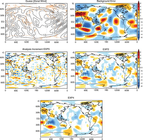
Fig. 9 Meridional wind (left column, ms−1) and geopotential height (right column, gpm) fields for (a, b) initial guess, (c, d) background error and (e, f) analysis increment for EXP4. As in figure 8, the background error is defined as true state minus background.
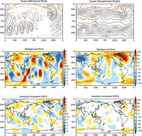
Fig. 10 Root mean squared error of guess vs. analysis fields for (a) zonal, (b) meridional wind (ms−1) and (c) geopotential height (gpm) fields within the assimilation window. The legends for lines are shown in (c).
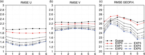
Fig. 11 Residual norm vs. the iteration number for optimisation.
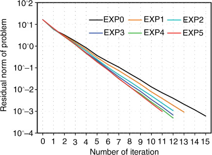
Table 1. Final observational cost function Jo and coefficient of the representer function for the 1st observation. The initial value for the observational cost function is Jo_initial=1996.2858000307174. The number of each iteration for convergence in the indirect method is parenthesised