
Figures & data
Table 1. DJF number of tracks that (K) had at least one point over 1500 m in Central Asia (30–55 N, 70–110°E), (K h ) were observed only over the elevated area, (K 0) were removed after topographic filtering even though they had some points below 1500 m, (K z ) remained in the list of tracks after topographic filtering
Fig. 1 Normalised annual histograms of (left column) the minimum central pressure (hPa) and (right column) the maximum cyclone deepening rate (hPa/6 h) for continental systems over regions where the topographic elevation is less than 1500 m (grey bars) and their deviations from the distribution for all continental cyclones when no elimination is applied (shown in colour). Note the scale difference between the climatological (right) and anomaly (left) axes.
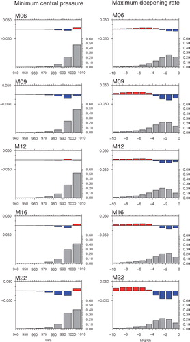
Fig. 2 DJF maps of characteristics of cyclones in M09 (left) and M12 (right) that had at least one point over the mountains in Central Asia: (a) cyclogenesis, (b) cyclolysis, (c) location of minimum SLP, (d) location of maximum deepening rate, (e) averaged deepening rate for all DJF cyclones (hPa/6 h). Counts in a–d show the number of systems per season in a circle of radius 2 deg. lat. The red line shows the 1500-m topography isoline.
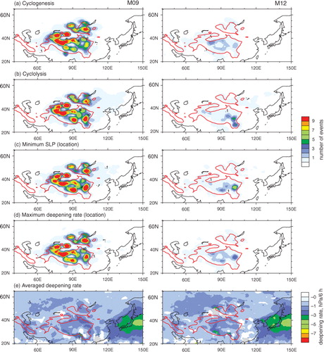
Fig. 3 Annual anomalies in the number of tracks that were reduced by 12 hours from the climatological number of tracks. The counts show the number of tracks per year in a circle of radius 2 deg. lat.
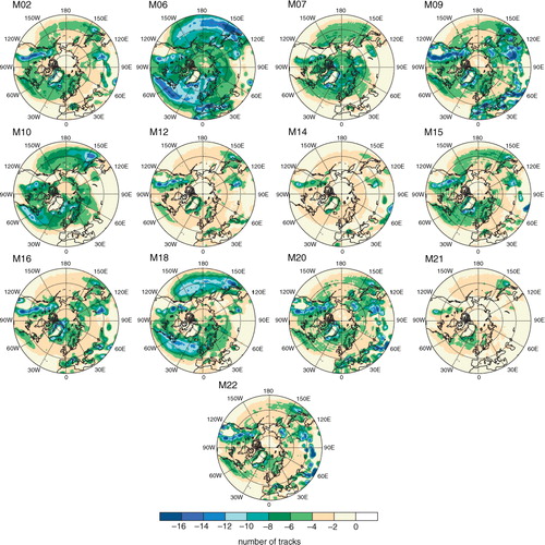
Fig. 4 (Left panel) Annual relative anomalies in the number of cyclones averaged across the schemes and (middle and right panel) two most contrasting examples after the first 12 hours of each track were removed. The counts show the number of tracks per year in a circle of radius 2 deg. lat. The red contour lines in the left panel show the standard deviation.
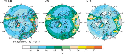
Fig. 5 Normalised annual climatological histograms of the maximum cyclone deepening rate (hPa/6 h) (; grey bars) along with the magnitudes of deviations of histograms implied by the truncation of the first 12 hours of cyclone tracks (
) from the original ones (
; colour bars).
=
–
.
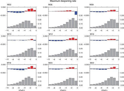
Table 2. Average duration of tracks before (LT) and after (LT12) the removal of the first 12 hours of each track (days) and difference between them (absolute, D LT , and normalised by LT, R LT )
Table 3. Number of RICs per scheme per 30-year period
Fig. 6 Distribution of (a) average and (b) maximum propagation speed of a cyclone centre.
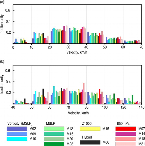
Fig. 7 (a) Tail of annual distribution of maximum propagation speed of a cyclone centre for tracks prior to orographic filtering and (b) spatial distribution of the number of tracking schemes that demonstrate a cyclone speed of 170 km/h and more. The counts show the number of tracking schemes in a circle of radius 2 deg. lat.
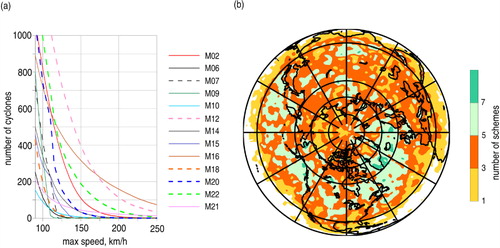
Table 4. Number of tracks (N) per scheme before splitting and the number of tracks that remained unchanged (R)
Fig. 8 Annual anomalies of the number of tracks that were split at their maximum propagation time step from the climatological number of tracks. The counts show the number of tracks per year in a circle of 2 deg. lat.
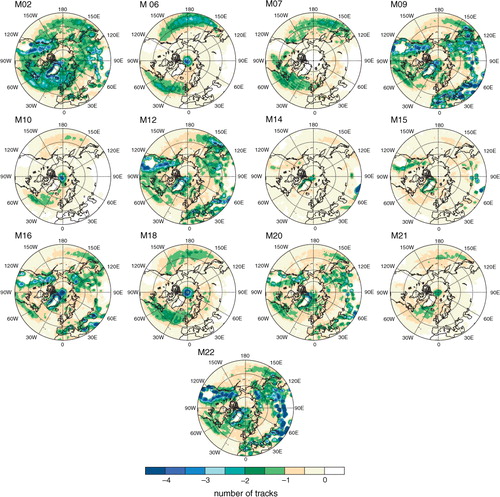
Fig. 9 DJF maps of (a) maximum deepening rate (hPa/6 h), (b) average deepening rate (hPa/6 h) and (c) average central pressure of cyclones (hPa). The left panels show average between the methods and middle and right panels show the two most contrasting schemes. The red contour lines show the STD.
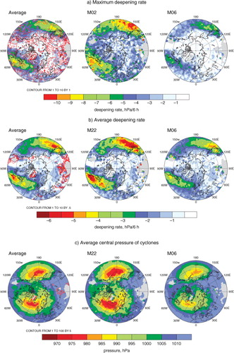
Fig. 10 DJF map of average central pressure of cyclones (hPa) for M02 and M10.
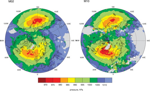
Fig. 11 (a) DJF and (b) JJA cumulative distribution for the number of tracks per season as a function of cyclone intensity (minimal central pressure). The plots are built using 10-hPa wide bins, and the dots are placed in the centre of the bins. (c) DJF and (d) JJA number of 200 most intense cyclone tracks averaged across the algorithms per each season (in colour). The counts show the number of tracks per year in a circle of 2 deg. lat. Red contour lines show STD.
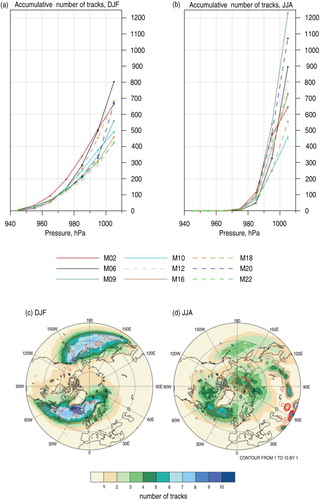
Table 5. The percentage of the total number of cyclones per season (DJF and JJA) which fall into the ‘200 most intense cyclones’ category (P 200) and the average SLP (hPa) in the centre of the 200th most intense cyclone in a season at the moment of its maximum intensity (SLP 200)
Table A1. Code numbers for the tracking methods used in this study, the main references for method descriptions and figures in which each method was used