A comparison of tracking methods for extreme cyclones in the Arctic basin

Figures & data

Fig. 1 (a) SLP pattern at 00 UTC 8 January 2002 when the lowest January central pressure was diagnosed (contour interval is 5 hPa). In the M10 scheme the centre of the cyclone was located at 5.1°E, 81.4°N (indicated in Figure) and had a central pressure was 938 hPa. (b) 300 hPa geopotential height at the same synoptic time (contour interval is 50 m).

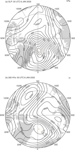
Table 1. Statistics the SLP cyclone with the lowest pressure (R1) in the 12 calendar months, for the period 1979–2009, with the time (UTC), date and year in which they occur, as determined by method M10

SLP cyclone				Z300 cyclone
Time	Date	Month	Year	Min. press. (hPa)	Anom.	Long. (°E)	Lat. (°N)	Min. Z300 (m)	Anom.	Long. (°E)	Lat. (°N)	Separation (km)
00	08	Jan	2002	938.0	−68.9	5.1	81.4	8222.5	−199.7	4.5	81.3	19.7
12	07	Feb	1995	946.8	−59.8	39.8	70.3	8101.0	−464.2	33.8	70.9	232.6
12	07	Mar	1997	947.3	−58.0	352.2	71.0	8301.2	−304.7	348.2	71.4	148.3
18	12	Apr	1990	953.5	−62.0	16.7	81.1	8254.1	−350.2	17.2	81.2	14.8
06	21	May	1998	964.9	−48.8	75.2	75.6	8508.5	−259.1	75.6	75.7	18.5
12	05	Jun	1994	970.2	−41.2	172.2	83.1	8494.6	−422.5	134.0	84.7	476.5
06	04	Jul	2002	974.5	−36.9	218.2	81.5	8587.2	−460.0	219.0	80.9	68.4
06	07	Aug	1995	966.7	−44.5	87.0	82.2	8650.0	−370.0	59.1	79.9	536.1
06	23	Sep	1982	957.7	−50.0	31.5	73.7	8635.5	−302.9	31.2	74.1	46.8
12	27	Oct	2003	950.9	−56.6	3.6	74.6	8408.0	−349.1	0.6	75.4	117.5
06	17	Nov	1996	942.5	−72.7	115.9	80.4	8123.8	−372.4	111.9	80.7	80.1
00	23	Dec	1990	940.6	−65.7	349.4	74.4	8241.5	−336.4	351.6	73.4	127.8

The fifth to eighth columns show the lowest central pressure, the deviation from the relevant monthly climatology at the location of the storm, and the longitude and latitude of the storm. The next four columns present analogous statistics for a vortex which was identified at the same time at the 300 hPa level in the vicinity of the surface storm. The last column displays the horizontal separation between the centres of the SLP and 300 hPa systems.

Fig. 2 Central pressure (hPa) of the R1, R2, R3, R4 and R5 cyclones in the 12 calendar months determined by each of the cyclone identification algorithms.

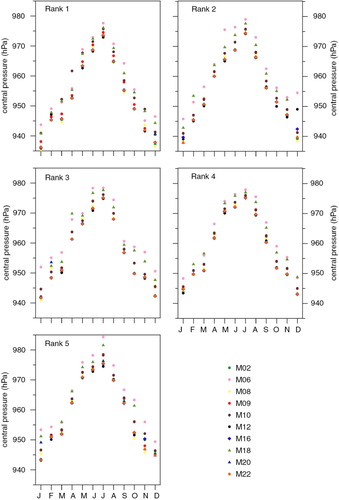
Fig. 3 Time series of the central pressure of cyclone identified in the methods in the time leading up to and after the minimum. The abscissa presents the time in days, and the zero represents the time of the minimum surface pressure.

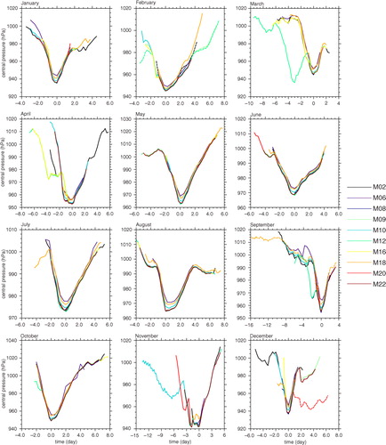
Table 2. Lifetime (in days) of the 12 R1 storms identified by the 10 identification methods

Mon	M02	M06	M08	M09	M10	M12	M16	M18	M20	M22	Max.		Ave.
Jan	8.25	4.75	3.50	3.75	5.00	4.25	4.00	5.50	4.00	3.50	8.25	M02	4.65
Feb	5.75	4.25	2.25	10.00	7.00	11.00	6.50	6.25	3.00	4.75	11.00	M12	6.07
Mar	8.50	6.25	2.00	2.50	2.25	9.00	8.75	6.00	2.50	2.25	9.00	M12	5.00
Apr	9.50	3.25	4.75	5.00	6.25	9.25	8.75	2.00	3.25	5.25	9.50	M02	5.72
May	6.25	6.25	6.25	9.75	7.25	10.25	7.25	7.00	9.75	9.75	10.25	M12	7.97
Jun	7.25	6.75	4.00	8.25	6.50	8.25	5.25	8.00	9.50	8.25	9.50	M20	7.20
Jul	8.25	7.25	6.50	6.50	3.25	6.75	6.75	9.25	6.50	6.50	9.25	M18	6.75
Aug	10.50	5.75	6.25	10.25	10.25	10.75	10.50	10.50	5.00	10.00	10.75	M12	8.98
Sep	12.00	9.75	8.75	3.25	10.25	7.75	3.00	19.50	4.75	5.00	19.50	M18	8.40
Oct	9.50	6.75	7.75	8.00	3.25	6.25	9.25	5.00	8.00	8.00	9.50	M02	7.18
Nov	7.00	1.75	1.50	7.50	17.25	9.00	−1	2.00	10.75	8.75	17.25	M10	7.28
Dec	7.75	2.75	2.00	6.00	3.50	−1	2.00	3.00	6.25	5.00	7.75	M02	4.25
Max	12.00	9.75	8.75	10.25	17.25	11.00	10.50	19.50	10.75	10.00
Sep	Sep	Sep	Aug	Nov	Feb	Aug	Sep	Nov	Aug
Ave	8.38	5.46	4.63	6.73	6.83	8.41	6.55	7.00	6.10	6.42

An unbiased estimate of lifetime is obtained by calculating N/4, where N is the number of consecutive (6-hourly) analyses in which the 12 storms are identified in the methods. Bold numbers denote the maximum for a given scheme, and Italics denotes the maximum for a given month, while Bold and italics indicate the maximum for a given month and scheme. Red font means that the cyclone was ranked the second or the third in that scheme, while ‘ −1’ indicates that the cyclone was not found in that scheme.

Fig. 4 Histogram of the frequency bins for the separation between the locations of minimum central pressure in the various cyclone methods. The distribution is drawn from all available comparisons for the top five ranked cyclones and for all 12 such months.

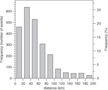
Table A1. Code numbers for the tracking methods used in this study, and the main references for method descriptions

Code	Main references for method description
M02	Murray and Simmonds (1991), Pinto et al. (2005)
M06	1997), Hewson and Titley (2010)
M08	2006)
M09	Serreze (1995), Wang et al. (2006)
M10	Murray and Simmonds (1991), Simmonds et al. (2003)
M12	2002), Rudeva and Gulev (2007)
M16	2002)
M18	1994, 1997)
M20	2006)
M22	2005), Akperov et al. (2007)

Fig. 5 Locations of the five most intense surface cyclones for each of the calendar months (filled circles). The five colours denote the five rankings (see legend). The crosses denote the location of a significant Z300 system within 1000 km of the surface cyclone.

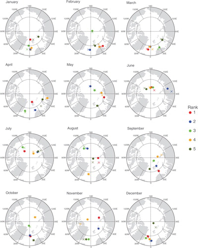
Table A2. Times and dates of the first, second, third, fourth and fifth highest ranked cyclone (R1, R2, R3, R4 and R5) for the 12 calendar months of the year

R1	R2	R3	R4	R5
Month	HH DD YYYY	HH DD YYYY	HH DD YYYY	HH DD YYYY	HH DD YYYY
Jan	00 08 2002	12 08 1993	12 11 1984	18 21 1994	00 13 2009
Feb	06 07 1995	18 06 1981	18 22 1996	18 28 1990	12 01 1993
Mar	12 07 1997	00 13 1995	00 01 1990	12 03 1979	12 22 2003
Apr	18 12 1990	18 04 2007	00 01 1995	00 04 1990	12 26 1997
May	00 21 1998	06 22 1992	18 02 1990	06 30 1994	06 04 2001
Jun	12 05 1994	12 19 1997	18 22 2008	12 08 1992	18 16 1986
Jul	06 04 2002	06 02 1986	18 29 2003	18 26 1992	18 05 1993
Aug	18 06 1995	18 28 1980	18 06 1991	00 22 1991	18 07 1994
Sep	06 23 1982	00 25 2003	06 28 1989	06 29 1986	12 02 1999
Oct	12 27 2003	18 12 1986	00 10 1988	18 28 1997	12 12 1996
Nov	06 17 1996	06 08 2004	12 10 2001	00 29 1993	06 28 1984
Dec	00 23 1990	00 20 1993	00 28 1980	12 23 2004	00 22 1979

‘HH’ denotes UTC time, ‘DD’ day of the month, and ‘YYYY’ year.

Murray R. J. , Simmonds I . A numerical scheme for tracking cyclone centres from digital data. Part I: development and operation of the scheme. Aust. Meteorol. Mag. 1991; 39: 155–166.

 Google Scholar

Pinto J. G. , Spangehl T. , Ulbrich U. , Speth P . Sensitivities of a cyclone detection and tracking algorithm: individual tracks and climatology. Meteorol. Z. 2005; 14: 823–838.

 Web of Science ®Google Scholar

Hewson T. D . Objective identification of frontal wave cyclones. Meteorol. Appl. 1997; 4: 311–315.

 Google Scholar

Hewson T. D. , Titley H. A . Objective identification, typing and tracking of the complete life-cycles of cyclonic features at high spatial resolution. Meteorol. Appl. 2010; 17: 355–381.

 Web of Science ®Google Scholar

Trigo I. F . Climatology and interannual variability of storm-tracks in the Euro-Atlantic sector: a comparison between ERA-40 and NCEP/NCAR reanalyses. Clim. Dyn. 2006; 26: 127–143.

 Web of Science ®Google Scholar

Wang X. L. , Swail V. R. , Zwiers F. W . Climatology and changes of extratropical cyclone activity: comparison of ERA-40 with NCEP-NCAR reanalysis for 1958–2001. J. Clim. 2006; 19: 3145–3166.

 Web of Science ®Google Scholar

Simmonds I. , Keay K. , Lim E.-P . Synoptic activity in the seas around Antarctica. Mon. Weather Rev. 2003; 131: 272–288.

 Web of Science ®Google Scholar

Zolina O. , Gulev S. K . Improving the accuracy of mapping cyclone numbers and frequencies. Mon. Weather Rev. 2002; 130: 748–759.

 Web of Science ®Google Scholar

Rudeva I. , Gulev S. K . Climatology of cyclone size characteristics and their changes during the cyclone life cycle. Mon. Weather Rev. 2007; 135: 2568–2587.

 Web of Science ®Google Scholar

Lionello P. , Dalan F. , Elvini E . Cyclones in the Mediterranean region: the present and the doubled CO2 climate scenarios. Clim. Res. 2002; 22: 147–159.

 Web of Science ®Google Scholar

Sinclair M. R . An objective cyclone climatology for the Southern Hemisphere. Mon. Weather Rev. 1994; 122: 2239–2256.

 Web of Science ®Google Scholar

Sinclair M. R . Objective identification of cyclones and their circulation intensity, and climatology. Weather Forecast. 1997; 12: 595–612.

 Web of Science ®Google Scholar

Wernli H. , Schwierz C . Surface cyclones in the ERA-40 dataset (1958–2001). Part I: novel identification method and global climatology. J. Atmos. Sci. 2006; 63: 2486–2507.

 Web of Science ®Google Scholar

Bardin M. Y. , Polonsky A. B . North Atlantic Oscillation and synoptic variability in the European–Atlantic region in winter. Izvest. Atmos. Ocean. Phys. 2005; 41: 127–136.

 Web of Science ®Google Scholar

Akperov M. G. , Bardin M. Y. , Volodin E. M. , Golitsyn G. S. , Mokhov I. I . Probability distributions for cyclones and anticyclones from the NCEP/NCAR reanalysis data and the INM RAS climate model. Izvest. Atmos. Ocean. Phys. 2007; 43: 705–712.

 Web of Science ®Google Scholar