Contrasting meridional structures of stratospheric and tropospheric planetary wave variability in the Northern Hemisphere

Figures & data

Fig. 1 (a) Zonal means of the standard deviations (m, blue thin line) of monthly 10 hPa eddy geopotential height anomalies (long-term mean seasonal cycle removed), the DFS representation of monthly height field (red dashed line), and zonal mean of the RMSD between the monthly observations and the DFS representation (black dashed line) from 1979 to 2009 over the NH extratropics. Panels (b)–(f) are the same as (a), but for 50, 100, 300, 500 and 700 hPa, respectively.

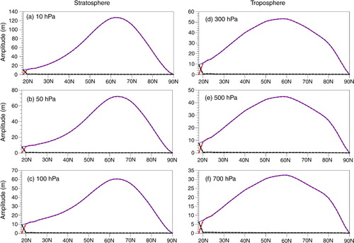
Fig. 2 (a) Climatological average over 31 (1979–2009) winters (DJF) of the wave amplitude as a function of k and l for the 10 hPa seasonal mean eddy geopotential height anomalies (long-term mean seasonal cycle removed) over the NH extratropics. The abscissa and ordinate represent zonal and meridional wavenumbers (k, l)=(1–5, 1–5), respectively. The amplitude values displayed in (a) have been divided by the maximum amplitude among all wave components (k, l). The maximum amplitude in (a) is 89 m for (k, l)=(1, 1). Panels (b)–(f) are the same as (a), but for 50, 100, 300, 500 and 700 hPa, respectively. The maximum amplitudes in (b)–(f) are 44 m for (k, l)=(1, 1), 24 m for (k, l)=(1, 1), 17 m for (k, l)=(1, 2), 14 m for (k, l)=(1, 2) and 11 m for (k, l)=(1, 2), respectively.

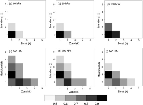
Fig. 3 (a) Time series of the amplitudes for 50 hPa wave patterns with zonal wavenumber 1 (k=1) and different meridional wavenumbers (l=1–3 denoted by red, blue and black lines, respectively) during the winters from 1979 to 2009. (b) As in (a), but for the 500 hPa wave patterns.

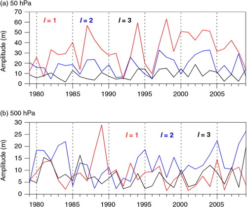
Table 1. Correlation coefficients for wave amplitude time series (k, l)=(1, 1–3) at 500 and 50 hPa between the NCEP2, NCEP1 and ERA-interim data sets during the winters of 1979–2009^a

l=1 at 500 (50) hPa	l=2 at 500 (50) hPa	l=3 at 500 (50) hPa
R(NCEP2, NCEP1)	0.95 (0.93)	0.96 (0.95)	0.94 (0.92)
R(NCEP2, ERA)	0.92 (0.89)	0.91 (0.88)	0.89 (0.87)
R(NCEP1, ERA)	0.90 (0.87)	0.89 (0.85)	0.86 (0.84)

^aAll correlation coefficients are statistically significant at the 95% confidence level.

Fig. 4 (a) Seasonal evolution of climatologically averaged (1979–2009) wave amplitude (k, l)=(1, 1–5) as a function of l and calendar month for the 50 hPa eddy geopotential height anomalies (long-term mean seasonal cycle removed) over the NH extratropics. The abscissa and ordinate represent calendar month and meridional wavenumber, respectively. The amplitude values displayed in (a) have been divided by the maximum amplitude among all sets of l and calendar month. The maximum amplitude in (a) is 50 m for l=1 and February. (b) As in (a), but for 500 hPa. The maximum amplitude in (b) is 16 m for l=2 and February.

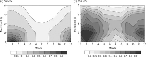
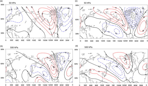
Fig. 5 The (a) first and (b) second EOFs (S-EOF1 and S-EOF2) of the 50 hPa winter NH eddy geopotential height anomalies (poleward of 20°N) for the period 1979–2009, shown as regressions of the height fields onto the normalised EOF time series. (c) Normalised time series of the S-EOF1 (red) and QBO (blue) indices for the winters from 1979 to 2009. (d) As in (c), but for the S-EOF2 (red) and ENSO (blue) indices.

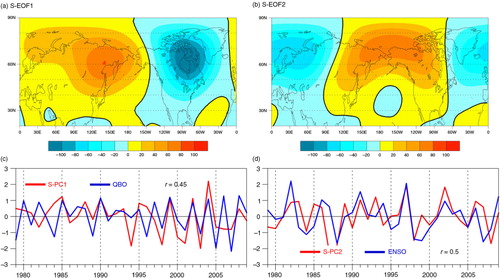
Fig. 6 Normalised wave amplitudes as a function of k and l for the 50 hPa eddy geopotential height anomaly associated with the (a) S-EOF1 and (b) S-EOF2 as shown in Fig. 5a and b. The abscissa and ordinate represent zonal and meridional wavenumbers, respectively.

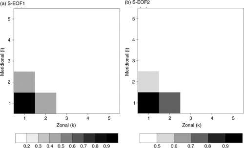
Fig. 7 (a) and (b) As in Fig. 4a and b, but for the leading two EOFs (T-EOF1 and T-EOF2) of the 500 hPa eddy geopotential height anomalies. (c) Normalised time series of the T-EOF1 (red) and ENSO (blue) indices for the winters from 1979 to 2009. (d) As in (c), but for the T-EOF2 (red) and NAO (blue) indices.

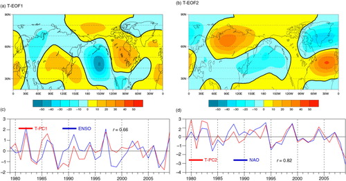
Fig. 8 Normalised wave amplitudes as a function of k and l for the 500 hPa eddy geopotential height anomalies associated with the (a) T-EOF1 and (b) T-EOF2 as shown in Fig. 7a and b. The abscissa and ordinate represent zonal and meridional wavenumbers, respectively.

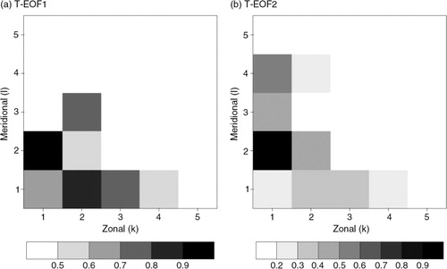
Fig. 9 (a) The vertical component of refractive index (m ²) for (k, l)=(1, 1) based on the DJF-mean zonal mean basic state in the NH. The index is scaled by a ²/10⁴. (b)–(d) as in (a), but for (k, l)=(2, 1), (k, l)=(1, 2), and (k, l)=(2, 2), respectively. In all the plots, regions with negative values are shaded.

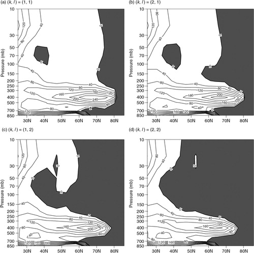
Fig. 10 (a) TM, (b) TV and (c) based on the DJF-mean zonal mean basic state in the NH extratropics. For the definitions and formulas of TM, TV and , see details in the text, and all of them are scaled by a ²/10 in the plots. In (c), regions with negative values are shaded.

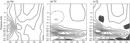
Fig. 11 (a) Vertical and (b) horizontal distributions of the tropical heating used in Exp1. Contour interval in (b) is 0.1° K d⁻¹. (c) Divergence at 200 hPa (in 10⁻⁷ s⁻¹) computed from the steady LBM response to the tropical heating in (a) and (b).

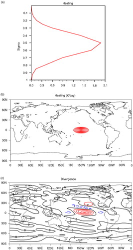
Fig. 12 The LBM simulated (a) stratospheric (sigma level equivalent to 50 hPa) and (b) tropospheric (sigma level equivalent to 500 hPa) responses of eddy geopotential height (in m) to the prescribed heating in Fig. 11. Linear barotropic model responses in eddy geopotential height (in m) to the tropical divergence forcing of Fig. 11c when linearised about the zonal mean flow at (c) 50 hPa and (d) 500 hPa. In all the barotropic experiments, the geopotential height was obtained by multiplying the streamfunction by the Coriolis parameter.