Midtropospheric frontogenesis associated with antecedent indirect precipitation ahead of tropical cyclones over the Korean Peninsula

Figures & data

Fig. 1 IR images from the GMS (upper panels) and rain rates (units: mm h⁻¹) from the Tropical Rainfall Measuring Mission (TRMM) 3B42 V6 data together with the effective radius of TC (middle panels) at the peak time of the first rainfall (red arrows in the bottom panels). The bottom panels show the time series of hourly precipitation from surface station recorded maximum precipitation in South Korea during the period associated with the TCs for the three AIP cases: Bart (1999; left), Saomai (2000; middle) and Soudelor (2003; right).

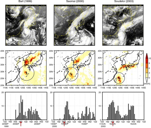
Fig. 2 Schematic of effective radius (R15) of TC, effective landfall time (LFT) and the station locations for direct precipitation (red crosses) and AIP (green crosses). Grey crosses denote the stations with no precipitation. Black line denotes TC track.

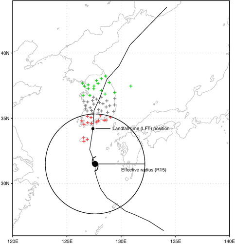
Fig. 3 Geopotential height (contour, units: gpm), QG frontogenesis [shading, units: 10⁻¹¹ K (m s)⁻¹] and horizontal winds (vector, units: m s⁻¹) at (a, b) 500 hPa, and (c, d) 925 hPa and (e, f) the meridional–vertical cross-section of QG frontogenesis, potential temperature (thick contour, units: K) and pressure velocity (thin contour, units: Pa s⁻¹) along 127.5°E at the maximum precipitation time for the representative two cases of RR-OT (Nari, 2007; left panel) and AIP (Saomai, 2000; right panel), respectively. The black triangle and TC symbol indicate the precipitating region and composite TC location, respectively.

Table 1. List of all documented AIP cases over the KP from 1993 to 2004

AIP – 23 cases
Year	TC name	LFT	T0	Precip	Stn	Diff
1993	PERCY	18Z29JUL	00Z29JUL	129	Suwon	18
1993	ROBYN	00Z10AUG	06Z08AUG	145	Jecheon	42
1993	YANCY	12Z03SEP	06Z02SEP	52	Seoul	30
1994	DOUG	06Z11AUG	12Z10AUG	90	Sokcho	30
1995	FAYE	06Z23JUL	06Z22JUL	110	Jeju	24
1995	JANIS	12Z26AUG	18Z24AUG	265	Boryeong	42
1995	RYAN*	18Z23SEP	00Z23SEP	109	Sokcho	18
1996	KIRK	00Z14AUG	12Z12AUG	72	Gwangju	36
1997	TINA	18Z08AUG	00Z07AUG	99	Mokpo	42
1998	YANNI*	06Z30SEP	18Z29SEP	103	Geoje	12
1999	OLGA	00Z03AUG	06Z02AUG	190	Yeongju	18
1999	ANN	12Z20SEP	12Z19SEP	159	Sanchoen	24
1999	BART	00Z24SEP	06Z23SEP	86	Uljin	18
2000	KAI-TAK	06Z11JUL	12Z10JUL	138	Haenam	18
2000	SAOMAI	18Z15SEP	00Z14SEP	72	Seosan	42
2002	RUSA	06Z31AUG	18Z30AUG	120	Gangneung	12
2003	LINFA*	00Z31MAY	18Z29MAY	88	Jangheung	30
2003	SOUDELOR	06Z19JUN	00Z18JUN	88	Seogwipo	30
2003	ETAU*	06Z08AUG	00Z07AUG	70	Cheonan	30
2003	MAEMI	12Z12SEP	18Z11SEP	142	Goheung	18
2004	MINDULLE	12Z04JUL	12Z03JUL	155	Gwangju	24
2004	MEGI	00Z19AUG	00Z18AUG	208	Jangheung	24
2004	SONGDA	00Z07SEP	00Z06SEP	46	Ulleungdo	24
Average				116.5		26.5

LFT: landfall time (see footnote in the text), T0: analysis time, Precip: maximum 6 h precipitation at the analysis time [units: mm (6 h)⁻¹], Stn: surface station at which maximum precipitation was recorded, Diff: time difference between LFT and T0 (units: h). The asterisk marks cases shared with remote rainfall cases suggested by Byun and Lee (2012).

Table 2. List of all documented non-AIP cases over the KP from 1993 to 2004

Non-AIP – 18 cases
Year	TC name	LFT	T0
1993	OFELIA	06Z27JUL	06Z26JUL
1994	WALT	00Z26JUL	00Z25JUL
1994	BRENDAN	00Z01AUG	00Z31JUL
1994	ELLIE	18Z13AUG	18Z12AUG
1994	SETH	18Z11OCT	18Z10OCT
1996	EVE	12Z18JUL	12Z17JUL
1997	ROSIE	00Z27JUL	00Z26JUL
1997	OLIWA	06Z16SEP	06Z15SEP
1998	ZEB	06Z17OCT	06Z16OCT
1999	NEIL	06Z27JUL	06Z26JUL
1999	PAUL	06Z07AUG	06Z06AUG
2000	BOLAVEN	00Z31JUL	06Z29JUL
2000	PRAPIROON	12Z31AUG	12Z30AUG
2002	RAMMASUN	00Z06JUL	00Z05JUL
2002	NAKRI	12Z13JUL	12Z12JUL
2002	FENGSHEN	12Z26JUL	12Z25JUL
2004	NAMTHEUN	00Z01AUG	00Z31JUL
2004	CHABA	06Z30AUG	06Z29AUG

TC name: parent TC of the non-AIP case; LFT: effective landfall time; T0: analysis time.

Table 3. Monthly occurrence numbers of AIP, non-AIP, and total cases and the monthly ratio of AIP to total (units: %)

	May	Jun	Jul	Aug	Sep	Oct	Total
AIP	1	1	4	9	8	0	23
Non-AIP	0	0	11	4	1	2	18
Total	1	1	15	13	9	2	41
Ratio (AIP/total, %)	100	100	26.6	69.2	88.9	0	58.5

Fig. 4 Locations (black TC symbols) and tracks (red line) of the TCs at the analysis time for (a) the AIP and (b) non-AIP cases. The black point and black circle denote mean location and mean effective size for each case, respectively.

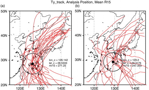
Fig. 5 Composite fields of geopotential height (black contour, units: gpm), temperature (red contour, units: K) at 200 hPa (a, b), 500 hPa (c, d) and 850 hPa (e, f) for the AIP (left panels) and non-AIP cases (right panels) at their respective analysis time. Shadings represent 200 hPa wind speed (units: m s⁻¹) in (a, b), 500 hPa horizontal winds (arrows, units: m s⁻¹) and convergence (units: 10⁻⁵ s⁻¹) in (c, d) and 850 hPa specific humidity (units: g kg⁻¹) in (e, f). Thick contours in (e, f) indicate the line at 1480 gpm. Dots denote the 90% significant region of the shading by the Student's t-test.

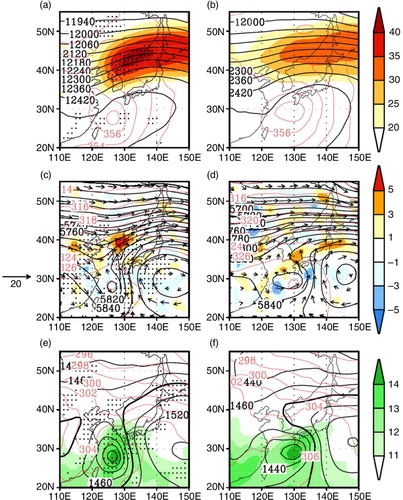
Fig. 6 Composite fields of (a) QG frontogenesis [shading, units: 10⁻¹¹ K (m s)⁻¹], streamline and omega (contour, negative dashed, units: Pa s⁻¹) averaged between 700 and 400 hPa, and (b) $\overrightarrow{Q}{\nabla }_p\theta$ (shading, units: 10⁻¹⁶ K² m⁻² s⁻¹), $\overrightarrow{Q}$ [vector, units: K (m s)⁻¹], $\overrightarrow{Q}$ convergence (contour, units: K m⁻² s⁻¹) at the analysis time. The dashed green (blue) rectangular indicates the frontal (ascending) region, which will be used for area-average (see the text). Colour shadings denote the 90% significant region of the shading by Student's t-test. The TC symbol indicates the composite TC location.

Fig. 7 Composite fields of various terms of the QG omega equation (shading, units: 10⁻¹² Pa m⁻² s⁻¹) and potential temperature (red contour, units: K) averaged between 700 and 400 hPa. (a) Three-dimensional Laplacian of composite omega [LHS of eq. (3)], (b) sum of all forcing terms [RHS of eq. (3)] (total forcing), (c) sum of QG forcing terms, (d) diabatic forcing terms, (e) differential geostrophic vorticity advection term and (f) the Laplacian of potential temperature advection term.

Fig. 8 Composite fields of (a) moisture flux (vector, units: m s⁻¹) and its convergence (shading, units: s⁻¹) averaged between 900 and 500 hPa at the analysis time, (b) meridional–vertical cross-section of specific humidity (shading, units: g kg⁻¹), moisture flux (vector) by meridional wind components (units: m s⁻¹) and negative pressure velocity (units: 30×Pas⁻¹), and meridional moisture flux convergence (contour, units: s⁻¹) along 127.5°E. Colour and green shadings denote the 90% significant region of the shading by Student's t-test. The TC symbol indicates the composite TC location and the triangle in (b) indicates the mean latitude (36.04°N) of surface stations in South Korea (i.e. the AIP region).

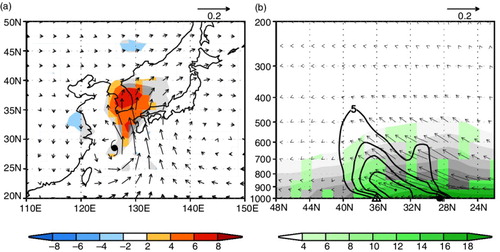
Fig. 9 Meridional–vertical cross-section of total frontogenesis (shading, units: 10⁻¹¹ K m⁻¹s⁻¹), potential temperature (thin contours, units: K) and pressure velocity (thick contours, units: Pas⁻¹) along 127.5°E. Arrows indicate the flow parallel to the cross-section (the horizontal component in m s⁻¹ and vertical component in 30 Pas⁻¹). Colour shadings denote the 90% significant region by Student's t-test. The TC symbol and triangle are the same as in Fig. 8.

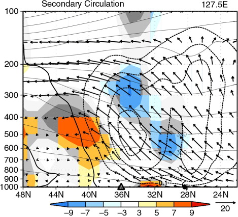
Fig. 10 Scatter plots: (a) between precipitation [units: mm (6 h) ⁻¹] averaged for all stations in South Korea and pressure velocity (units: Pas ⁻¹) averaged over the ascending region (blue box in Fig. 6a), (b) between QG frontogenesis (units: 10 ⁻¹¹ K m ⁻¹ s ⁻¹) averaged over the frontal region (green box in Fig. 6a) and pressure velocity and (c) between QG frontogenesis and precipitation. All plots use the values at the analysis time.

Fig. 11 Schematic diagram for the physical processes associated with the AIP event over the KP.

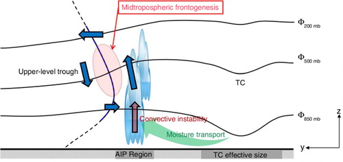
Fig. 12 Composite fields of geopotential height (contour, units: gpm), QG frontogenesis [shading, units: 10⁻¹¹K (m s)⁻¹] and horizontal winds (vector, units: m s⁻¹) at (a) 200 hPa, (b) 500 hPa and (c) 925 hPa for the AIP cases at the analysis time. The colour shadings and thick arrows represent the 90% significant region by Student's t-test.

Fig. 13 Geopotential height (contour, units: gpm), QG frontogenesis [shading, units: 10⁻¹¹ K (m s)⁻¹] and horizontal winds (vector, units: m s⁻¹) at (a, b, c) 200 hPa, (d, e, f) 500 hPa, and (g, h, i) 925 hPa and (j, k, l) meridional–vertical cross-section of QG frontogenesis, potential temperature (thick contours, units: K) and pressure velocity (thin contours, units: Pa s⁻¹) along 127.5°E at the maximum precipitation time for the composite fields of AIP (left panel), RR-OT (middle panel) and PRE-SJ (right panel), respectively. The black triangle and TC symbol in the bottom panel indicate the precipitating region and composite TC location, respectively.

Table 4. Summary of relevant characteristics of TC and frontogenesis among the AIP, RRE, and PRE cases

	AIP	RR-OT	PRE-SJ
Averaging distance between TC and rainfall region	~880 km	~1140 km	~830 km
TC intensity	Strong	Weak	Weak
Level of wind balance between TC and mid-latitude westerlies	Mid-level	Do not interact	Low level
Frontogenesis	Midtropospheric frontogenesis	Pre-existing surface frontogenesis	Surface frontogenesis

Byun K.-Y. , Lee T.-Y . Remote effects of tropical cyclones on heavy rainfall over the Korean peninsula – statistical and composite analysis. Tellus. 2012; 64: 14983.

 Google Scholar