
Figures & data
Fig. 1 Uniformly distributed coarse-resolution innovations (c-inno) plotted by blue+signs, and high-resolution innovations (h-inno) plotted by purple x signs. The solid black curve plots the benchmark analysis increment Δa. The dashed red curve plots the analysis increment Δa 20 from SE with 20 iterations. The solid green curve plots the analysis increment Δa I-20 from the first step of two-step experiment (TEA, TEB or TEC) with 20 iterations. The dashed blue, dotted cyan and dot-dashed grey curves plot the analysis increments Δa A20 from TEA, Δa B20 from TEB and Δa C20 from TEC, respectively, with 20 iterations.
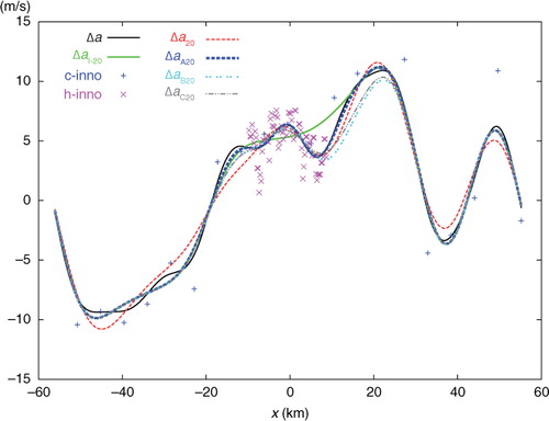
Fig. 2 C b(x) plotted by red curve and C a(x) plotted by dotted blue curve.
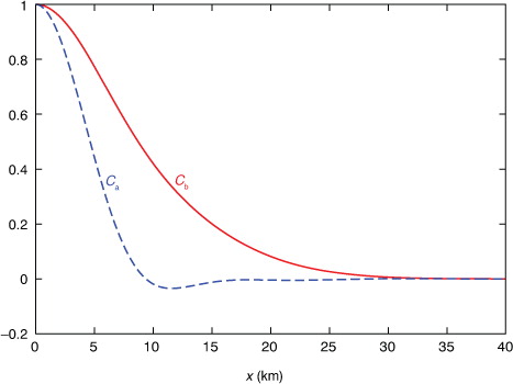
Fig. 3 Discrete background error power spectrum S(k i ) (that forms the diagonal matrix S) plotted by red+signs, and discrete analysis error power spectrum S a(k i ) (that forms the diagonal part of S a) plotted by green×signs, where k i =iΔk and Δk≡2π/D=5.7×10−5 m−1. The solid red (or green) curve plots S(k) [or S a(k)], that is, the continuous counterpart of S(k i ) [or S a(k i )] in the limit of D=NΔx→∞ for fixed Δx.
![Fig. 3 Discrete background error power spectrum S(k i ) (that forms the diagonal matrix S) plotted by red+signs, and discrete analysis error power spectrum S a(k i ) (that forms the diagonal part of S a) plotted by green×signs, where k i =iΔk and Δk≡2π/D=5.7×10−5 m−1. The solid red (or green) curve plots S(k) [or S a(k)], that is, the continuous counterpart of S(k i ) [or S a(k i )] in the limit of D=NΔx→∞ for fixed Δx.](/cms/asset/a2273cdf-262f-4ed5-85ab-a967b97cef69/zela_a_11830317_f0003_ob.jpg)
Fig. 4 (a) Full-matrix structure of S a. (b) Magnified structure of S a. The coloured contours plot the element value in m2s−2.
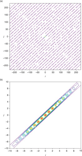
Fig. 5 (a) Structure of benchmark A plotted by colour contours every 0.5 m2s−2. (b) Deviation of approximately calculated A from benchmark A plotted by solid (or dashed) contours at 0.01 (or −0.01) m2s−2. The deviation in (b) reaches the maximum (or minimum) of 0.01156 (−0.01145) m2s−2 at the point marked by the +(or −) sign on the diagonal, and this diagonal point corresponds to a grid point that is collocated with a coarse-resolution innovation (or located in the middle between two adjacent coarse-resolution innovations).
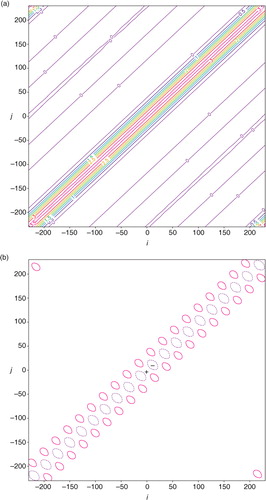
Fig. 6 Analysis error e 20 (or e 100) from SE with 20 (or 100) iterations plotted by dashed (or solid) red curve, analysis error e A20 (or e A100) from TEA with 20 (or 100) iterations plotted by dashed (or solid) blue curve, and analysis error e B20 (or e C20) from TEB (or TEC) with 20 iterations plotted by dot-dashed cyan (or grey) curve.
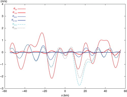
Table 1. Entire-domain averaged RMS errors (in ms−1) for the analysis increments obtained from SE, Step-I, TEA, TEB and TEC applied to the first set of innovations with periodic extension and consecutively increased n, where n is the number of iterations and Step-I stands for the first-step analysis (in TEA, TEB or TEC). All the RMS errors are evaluated with respect to the benchmark analysis increment Δa except for those in the third row where the RMS errors are evaluated versus Δa I – the benchmark for the first-step analysis itself, obtained directly from eq. (1a) for the coarse-resolution innovations only
Fig. 7 As in but for the non-uniform coarse-resolution innovations in the second set. The contours in (a) are plotted every 1 m2s−2. The contours in (b) are plotted at ±0.2, ±0.5 and −1 m2s−2. The deviation in (b) reaches the maximum value of 0.639 m2s−2 (or minimum value of −1.131 m2s−2) at the diagonal point marked by the +(or −) sign.
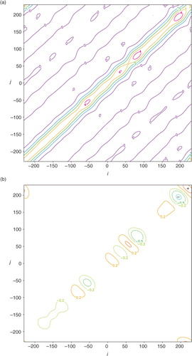
Fig. 8 As in but for the second set of innovations. The dotted green (or purple) curve plots C a+(x) [or C a− (x)] – the correlation structure intercepted from the benchmark A in a across the point marked by the +(or −) sign in b.
![Fig. 8 As in Fig. 2 but for the second set of innovations. The dotted green (or purple) curve plots C a+(x) [or C a− (x)] – the correlation structure intercepted from the benchmark A in Fig. 7a across the point marked by the +(or −) sign in Fig. 7b.](/cms/asset/cb33233f-6555-4031-9073-3f2c918fd8b0/zela_a_11830317_f0008_ob.jpg)
Fig. 9 As in but for the second set of innovations.
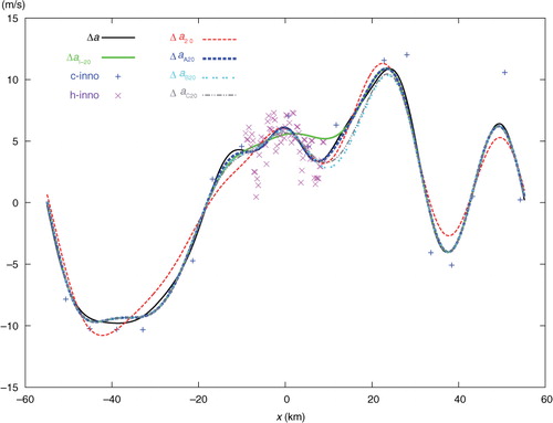
Fig. 10 As in but for the second set of innovations.
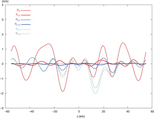
Table 2. As in but for the second set of innovations with periodic extension
Fig. 11 As in but without periodic extension. The contours in (b) are plotted at ±0.2, ±0.5, ±1, ±3, −5 and −7 m2s−2.
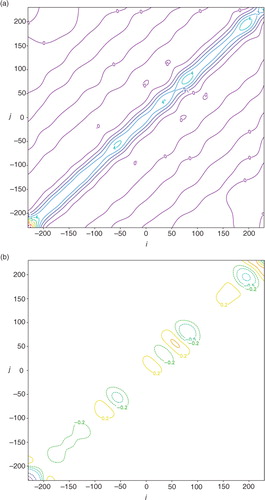
Fig. 12 As in but without periodic extension.
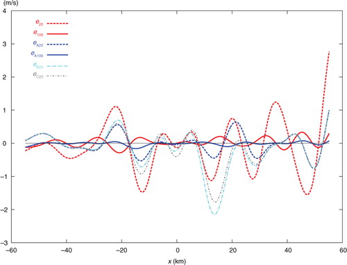
Table 3. As in but without periodic extension
Fig. 13 (a) Uniformly distributed coarse-resolution innovation points plotted by red+signs over the analysis domain, and high-resolution innovation points plotted by the green dots in the nested domain of D x /6=20 km long and D y /6=10 km wide. (b) As in (a) but for the second set in which the coarse-resolution innovations are not uniformly distributed. The coarse-resolution innovations in (a) are spaced every Δx co=6 km (or Δy co=6 km) in the x-direction (or y-direction). The domain-averaged resolution for the non-uniformly distributed coarse-resolution innovations in (b) is estimated also by Δx co ≈ 6 km (or Δy co ≈ 6 km) in the x-direction (or y-direction).
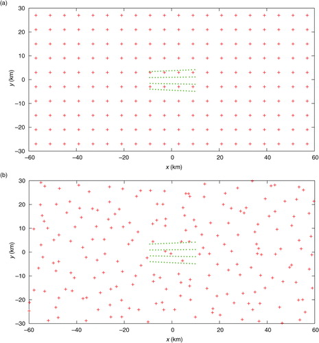
Fig. 14 C a(x−x c) plotted by the green contours for x c=(0, 0), and benchmark correlation pattern plotted by the black contours with x c also placed at x=(0, 0) – the centre of the analysis domain. Here, x c denotes the correlation centre.
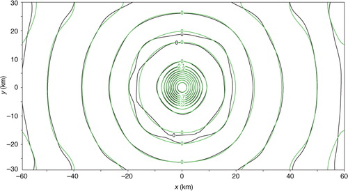
Fig. 15 Deviation of σ e 2 (= 3.1527 m2s−2) from benchmark analysis error variance plotted by contours at 0, ±0.05, −0.1, −0.2, −0.5, −1, −3 and −5 m2s−2 over the analysis domain.
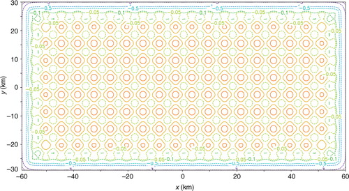
Fig. 16 Benchmark analysis increment Δa plotted by black contours, analysis increment Δa 20 from SE with 20 iterations plotted by red contours, and analysis increment Δa A20 from TEA with 20 iterations plotted by blue contours. The rectangle plotted by thin black lines shows the nested domain.
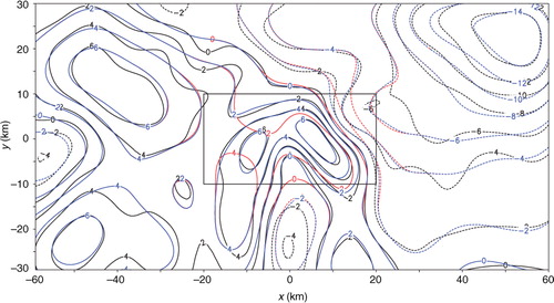
Fig. 17 Analysis error e 20 from SE and analysis error e A20 from TEA with 20 iterations plotted by red and blue contours, respectively. The rectangle plotted by thin black lines shows the nested domain.
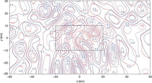
Table 4. As in but for the first set of innovations in the two-dimensional case as shown in a
Fig. 18 As in but for the second set of innovations.
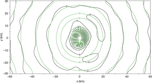
Fig. 19 As in but for the second set of innovations with contours plotted every 1 m2s−2.
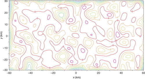
Fig. 20 As in for the second set of innovations.
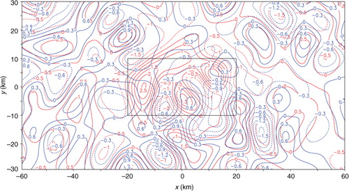
Table 5. As in but for the second set of innovations as shown in b