Multiple equilibria on planet Dune: climate–vegetation dynamics on a sandy planet

Figures & data

Fig. 1.  Schematics of the model structure, and list of model variables.

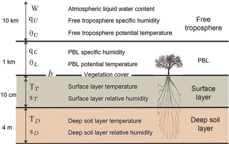
Fig. 2.  Panel (a) shows a scheme of the energy balance: incoming solar radiation travels through the atmosphere, which is transparent to short-wave radiation, but a part of it is reflected by clouds. Surface heating depends on the surface albedo, which is a function of vegetation cover. The surface layer emits long-wave (infrared) radiation upwards. Arrows in the atmosphere show absorption/emission of thermal radiation by the different layers. Panel (b) shows a scheme of the water cycle. Water vapour in the PBL is uplifted by convective fluxes. Water then may condensate in the free troposphere and precipitate as rainfall. Evapotranspiration has the essential role of transferring water back into the atmosphere. Without this effect, the deep soil reservoir would not take part in the cycle, and after some losses water would remain stored there.

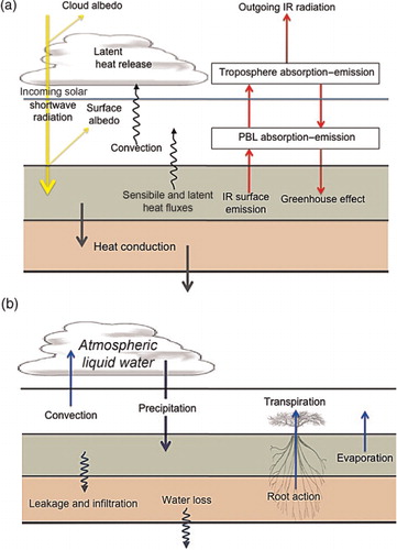
Table 1. Parameter names, symbols, values and unit of measurements

Symbol	Meaning	Value	Unit
Le	Specific latent heat of evaporation	2.501·10^6	J kg^−1
cp	Air specific heat	1000	J kg^−1 K^−1
cps	Soil specific heat	1000	kg m^−3
ρ U	Air density in the upper atmospheric layer	0.720	kg m^−3
ρ L	Air density of PBL	1.200	kg m^−3
ρ W	Water density	1000	kg m^−3
ρ s	Soil density	1800	kg m^−3
hU	Thickness of upper atmospheric layer	10000	m
hL	Thickness of PBL	1000	m
ZT	Depth of surface soil layer	0.1	m
ZD	Depth of deep soil layer	4.0	m
Z 0	Depth of bottom soil layer	10.0	m
n	Soil porosity	0.4
W 0	Maximum water content in the atmosphere before precipitation	5.0	kg m^−2
β	Ratio between sensible and latent convective heat flux	2
ɛ U	Free troposphere absorption/emission coefficient	0.25
ɛ L	PBL absorption/emission coefficient	0.22
ɛ W	Liquid water absorption/emission coefficient	0.6
ɛ S	Soil absorption/emission coefficient	0.85
α e	Albedo of bare soil	0.25
α v	Albedo of vegetated soil	0.18
S	Shading effect coefficient	0.5
	Timescale for temperature relaxation between surface and deep soil layer	180	d
	Timescale for temperature relaxation between deep soil layer and the soil below	360	d

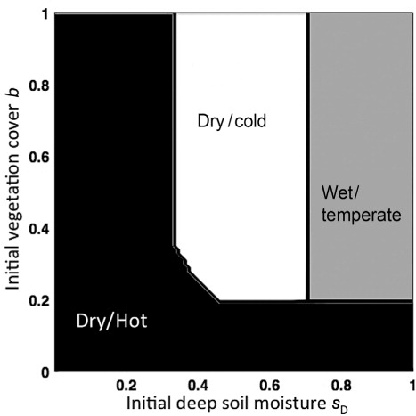
Fig. 3.  Equilibrium potential temperature in the PBL for the parameter values indicated in the Appendix, as a function of the initial conditions on s _D (x-axis) and on b (y-axis). The black area indicates the equilibrium state (dry and hot, ), the white area indicates state (dry and cold, ), and the grey area indicate state (wet and temperate, ).

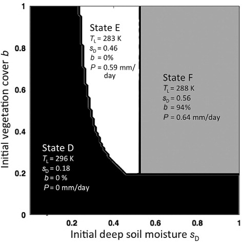
Fig. 4.  Temporal dynamics of vegetation cover, starting from different initial conditions of deep soil moisture s _D and vegetation cover b, and reaching three different states: (red dashed line), (green continuous line), and (blue dotted line). Note the different timescales needed to reach the various states. In these simulations, initial conditions used to reach state are s _Di =0.6, and b _i =0.1; state , s _Di =0.5, and b _i =0.5; state , s _Di =0.6, and b _i =0.4.

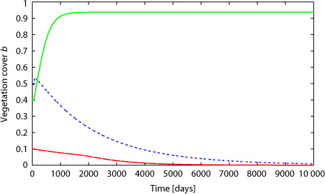
Fig. 5.  Contour plot showing different θ _L values in the three stable states, as in Fig. 3, but with a root depth Z _D =1 m. In this case, the water available for the system is much less than in the standard configuration, therefore the wet/temperate state is reached only with larger initial values of s _D and b. The black area indicates the state , the white area the state and the grey area the state .