Figures & data
Table 1. Planetary greenhouse parameters
Table 2. Single-addition and single-subtraction normalised LW greenhouse flux attribution (after Lacis et al., 2010)
Fig. 1 Global maps and seasonal change of the greenhouse effect for 1850 (left panels) and 2000 (right panels). The magnitude of the greenhouse effect has increased by about 6 W m−2 since 1850, but the geographical patterns are largely unchanged. The seasonal change in greenhouse strength (12 W m−2) also remains invariant, but it is twice as large as the secular trend. The seasonal change in greenhouse strength is largest over land areas, and it is affected by changes in surface temperature and seasonal shifts in water vapour and cloud distributions. The greenhouse strength is near zero in the Polar Regions, with negative values occurring over Antarctica during the winter season due to large temperature inversions.
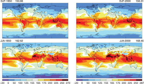
Fig. 2 Time trend of the terrestrial greenhouse effect from 1850 to 2010 from a 5-run ensemble average using the GISS 40-layer 2°×2.5° ModelE coupled atmosphere-ocean model. The 3-D 26-layer ocean model generates El Nino-like inter-annual variability. Also evident are the effects of major volcanic eruptions. These are denoted by the heavy black arrows for the major volcanoes (Shiveluch, Krakatoa, Santa Maria, Agung, El Chichon, Pinatubo). The shape of the greenhouse trend has a strong resemblance to the time trend of the non-condensing greenhouse gases for the same time period.
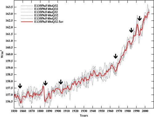
Fig. 3 Hourly model diagnostic results for the ‘virtual’ forcing of climate by instantaneous water vapour changes. There is rapid convergence to equilibrium following instantaneous doubling and zeroing of atmospheric water vapour. The left-hand panels show global-mean water vapour at 299 and 974 mb level converging to control run equilibrium values. The right-hand panels show the upwelling longwave (LW) flux at the top (TOA) and the bottom (BOA) of the atmosphere. Diurnal oscillations in the global-mean LW flux arise from the diurnal surface temperature change over land areas. Red curves depict the model response to doubled water vapour amounts. The green curves refer to the model response to zeroed water vapour. The blue curves are for the control run water vapour reference results. Water vapour changes in the left-hand panels have been normalised relative to the control run results.
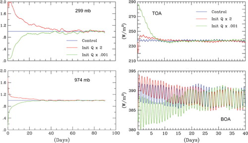
Fig. 4 Hourly model diagnostics of the globally averaged greenhouse effect convergence to equilibrium following the instantaneous doubling (red) and zeroing (green) of atmospheric water vapour. Diurnal oscillations in the globally averaged greenhouse strength result from land-ocean differences in diurnal surface temperature changes. Convergence to equilibrium is fastest for the doubled water vapour experiment since relative humidity above 100% leads to rapid condensation and rain-out. The Clausius–Clapeyron relation is basic to establishing the equilibrium atmospheric water vapour distribution. The reference atmosphere of the time scale zero point is 1 December 1949, which is comparable to the DJF 1850 greenhouse strength in .
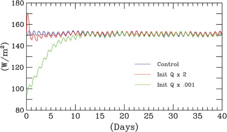
Fig. 5 Basic principles for transmission, absorption and emission of thermal radiation: Kirchhoff's law of thermal radiation.
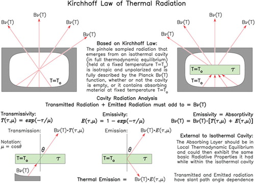
Fig. 6 Thermal emission from homogeneous layer with linear-in-Planck temperature gradient.
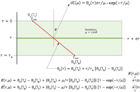
Fig. 7 Schematic outline for computation of monochromatic longwave (LW) fluxes and cooling rates.
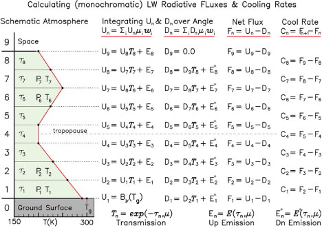
Fig. 8 Upward (top) and downward (bottom) spectral fluxes in clear-sky standard atmosphere.
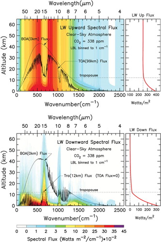
Fig. 9 Clear-sky case spectral net flux (top panel) and spectral cooling rate (bottom panel).
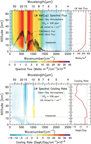
Fig. 10 Spectral net flux change (top) and spectral cooling (bottom) for doubled CO2.
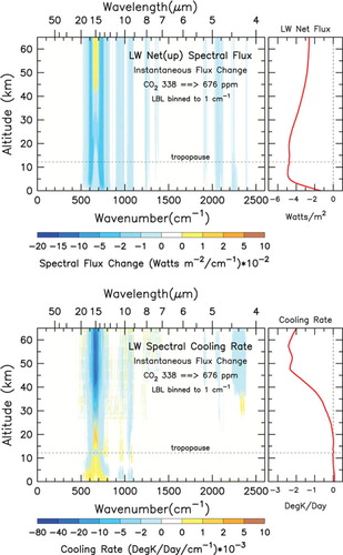
Fig. 11 Line-by-line (LBL) and 3-D general circulation climate model (GCM) radiative flux and cooling rate comparisons for Mid-Latitude Atmosphere calculations. Reference LBL calculations are depicted in red. GISS ModelE calculations using the correlated k-distribution methodology are plotted in black (on top of the red lines). Left-hand panel shows virtual agreement for the downwelling and upwelling fluxes. Cooling rates are shown in the middle panel, with flux differences plotted at right. The 33 spectrally non-contiguous correlated k-distribution intervals in the GCM radiation model are able to closely reproduce the LBL calculation results that utilise over 107 spectral points. For comparison, the dotted lines depict the corresponding results for the vintage 25-k interval GCM radiation model from Hansen et al. (Citation1988), which is used in the climate-forcing calculations for extreme CO2 amounts described in Section 6.
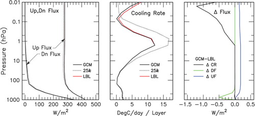
Fig. 12 Geological record of climate forcings, temperature, sea level and surface albedo response. (a) CO2 and CH4 data are derived from the Antarctic Dome C ice-core analysis, sea-level record based on analysis of Bintanja et al. (Citation2005). (b) Greenhouse gas and surface albedo forcing are from GCM modelling studies, with ice sheet area inferred from sea-level changes. (c) Dome-C-derived temperature change has been divided by two to represent global-mean temperature change. The calculated temperature change is based on a fast-feedback climate sensitivity of 0.75°C per W m−2, as per 3°C for doubled CO2. (after Hansen et al., Citation2008)
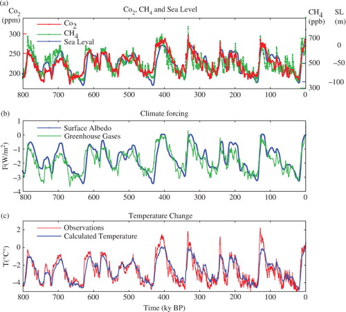
Fig. 13 Global energy balance analysis using global equilibrium surface temperature comparisons over an extended range of CO2 radiative forcing. At the left is the energy input scale (W m−2) with red arrows designating solar energy input. Heavy blue arrows represent outgoing energy [reflected solar, and longwave (LW) TOA flux to space]. The temperature scale in the figure interior gives the surface temperature (°C). The right-hand scale is for effective temperature (K). The pink region, covering the range of successive CO2 doublings, is the absorbed solar radiation (W m−2). The green region represents the radiative forcing caused by the successive CO2 doublings. The yellow region depicts the water vapour and cloud fast-feedback contribution (W m−2) to the total greenhouse strength. At bottom right, minor non-solar sources of energy input to the global climate system are shown in equivalent effective temperature units. The heavy red arrow angling towards figure top depicts a possible ‘runaway’ danger zone where positive CO2 feedbacks from existing CO2 reservoirs have the potential to exceed human capacity to maintain control over global climate change. Model results were calculated using the Russell et al. (Citation2013) 27-layer, 4°×3° coupled fast atmosphere-ocean model (FAOM). Based on attribution analysis, the feedback contribution to the greenhouse strength (yellow) is subdivided into its water vapour and cloud components. Similarly, the radiative forcing contribution to the greenhouse strength (green) is subdivided into CO2 and other GHG contributions. Similarly, the absorbed solar radiation (pink) is subdivided into portions that are absorbed within the atmosphere and solar radiation that is absorbed by the ground surface. The Effective Temperature and Surface Energy scales coincide numerically at zero, and also at the common point where 260.3 K=260.3 W/m2, connected otherwise by slanted lines.
![Fig. 13 Global energy balance analysis using global equilibrium surface temperature comparisons over an extended range of CO2 radiative forcing. At the left is the energy input scale (W m−2) with red arrows designating solar energy input. Heavy blue arrows represent outgoing energy [reflected solar, and longwave (LW) TOA flux to space]. The temperature scale in the figure interior gives the surface temperature (°C). The right-hand scale is for effective temperature (K). The pink region, covering the range of successive CO2 doublings, is the absorbed solar radiation (W m−2). The green region represents the radiative forcing caused by the successive CO2 doublings. The yellow region depicts the water vapour and cloud fast-feedback contribution (W m−2) to the total greenhouse strength. At bottom right, minor non-solar sources of energy input to the global climate system are shown in equivalent effective temperature units. The heavy red arrow angling towards figure top depicts a possible ‘runaway’ danger zone where positive CO2 feedbacks from existing CO2 reservoirs have the potential to exceed human capacity to maintain control over global climate change. Model results were calculated using the Russell et al. (Citation2013) 27-layer, 4°×3° coupled fast atmosphere-ocean model (FAOM). Based on attribution analysis, the feedback contribution to the greenhouse strength (yellow) is subdivided into its water vapour and cloud components. Similarly, the radiative forcing contribution to the greenhouse strength (green) is subdivided into CO2 and other GHG contributions. Similarly, the absorbed solar radiation (pink) is subdivided into portions that are absorbed within the atmosphere and solar radiation that is absorbed by the ground surface. The Effective Temperature and Surface Energy scales coincide numerically at zero, and also at the common point where 260.3 K=260.3 W/m2, connected otherwise by slanted lines.](/cms/asset/f8ef8c89-8620-49e8-837f-8d807bf31fcf/zelb_a_11817248_f0013_ob.jpg)
Table 3. LW greenhouse effect (GF) fractional attribution
Table 4. SW solar reflected/absorbed fractional attribution