Figures & data
Fig. 1 Location of monitoring stations in Santiago's air quality network since the 1980's (for details see text). The symbols correspond to the names of the stations A: Gotuzzo, B: Providencia (not used in this study, in white), F: Independencia, L: La Florida, M: Las Condes, N: Parque O'Higgins, O: Pudahuel, P: Cerrillos, Q: El Bosque (seven stations continuously working on the period 1997–2008, in grey), R: Cerro Navia, S: Puente Alto, T: Talagante, V: Quilicura (four more stations added on the period 2009–2010, in black). The limit of the current urban area is indicated by a heavy line. Main topographic features of the Santiago basin are also shown.
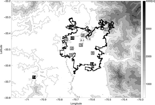
Table 1 Description of the air quality monitoring stations belonging over time to Santiago's monitoring network and the two periods of data used in this study.
Table 2 Relative quadratic error in percentage using different statistical models for fitting the 1997–2008 data for 7 stations and 4 measured species and for the 2009–2010 data for 11 stations and 3 measured species.
Fig. 2 Schematic evolution of the total information of the network.
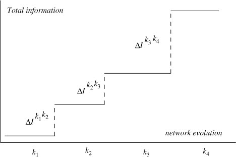
Table 3 Main statistics (mean, standard deviation and maximum) for each of the 7 monitoring stations working during the period 1997–2008 based on hourly averages during all the year (All), summer (S: Dec, Jan, Feb) and winter (W: Jun, Jul, Aug).
Table 4 Main statistics (mean, standard deviation and maximum) for each of the 11 monitoring stations working during the period 2009–2010 based on hourly averages during all the year (All), summer (S: Dec, Jan, Feb) and winter (W: Jun, Jul, Aug).
Table 5 Percentage of available hourly data considering 7 stations (period 1997–2008) and 11 stations (period 2009–2010) for all years and months (All), summer (S: Dec, Jan, Feb) and winter (W: Jun, Jul, Aug).
Fig. 3 Example of some statistical fitting. PM10 in winter for station N and O3 for stations M for normal (top line), log-normal (middle line) and gamma (bottom line) fitting. The relative quadratic error is indicated on each case.
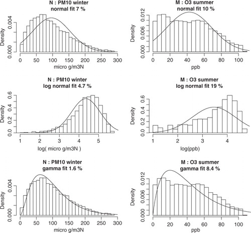
Fig. 4 Specificity (left) and representativity (right) for the univariate case for CO, O3, PM10, and SO2 for summer for seven stations during 1997–2008. The larger the circle, the larger the index.
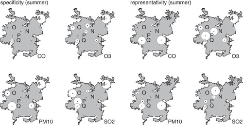
Fig. 5 Specificity (left) and representativity (right) for the univariate case for CO, O3, PM10 and SO2 for winter for seven stations during 1997–2008. The larger the circle the larger the index.
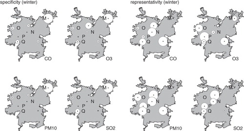
Fig. 6 Evolution of ‘specificity’ (upper panels) and ‘representativity’ (lower panels) indexes for PM10 in winter and O3 in summer respectively. See text for details.
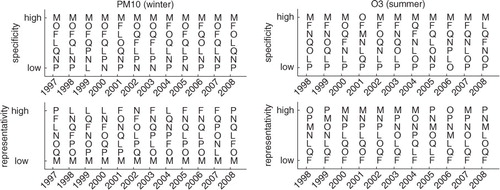
Fig. 7 Multivariate specificity (top) and representativity (bottom) indexes for simultaneously CO, O3, PM10 and SO2 for hourly data for the period 1997–2008 separately for summer, winter and all seasons.
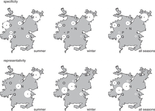
Fig. 8 Evolution of total information content of the air quality monitoring network in Santiago since the late 1980s relative to the current situation, considering PM2.5.
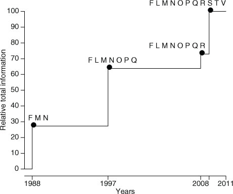
Fig. 9 Simulated interpolation of the measurements at some sites (×) from the available network (•) using Barnes interpolation (here for some typical log concentrations of PM10 in greyscale, lighter=higher). To localise, we put 12 phantom zero measurement stations around the boundary. This allows to better estimate the a priori mean and covariances B
i
for the evolution of network total information taking into account the spatial distribution.
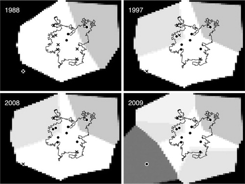
Fig. 10 Evolution of total information content of the air quality monitoring network in Santiago since the late 1980s relative to the current situation, considering PM2.5 using Barnes interpolation a priori information.
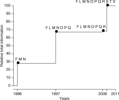
Fig. 11 Information gain map. At each point, the difference in information gain obtained by comparison of the total information gain of the original network and the total information gain obtained for a new network after adding a new station at this point with Barnes's interpolated values is indicated.
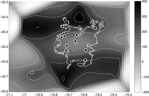
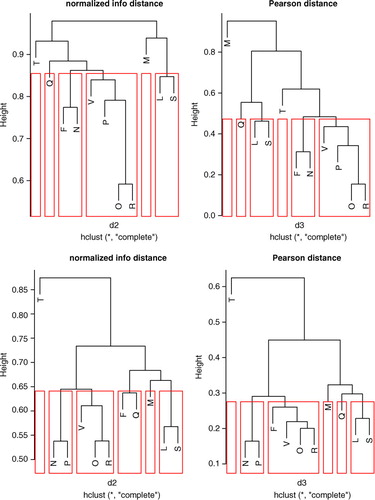
Fig. 12 Hierarchical clustering following the (not normal) normalised information distance (left column) defined in (8) compared with the Pearson correlation function (right column) for PM2.5 (top line) and O3 (bottom line).