How will land use affect air temperature in the surface boundary layer? Lessons learned from a comparative study on the energy balance of an oak savanna and annual grassland in California, USA

Figures & data

Fig. 1 Image of the field sites under investigation. The Tonzi Ranch is the venue of the oak savanna flux tower. The annual grassland is located on the Vaira Ranch. Both sites are near Ione, CA.

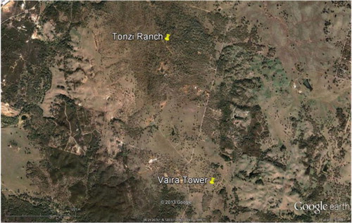
Fig. 2 A comparison in daily-averaged potential air temperature an annual grassland and savanna ecosystem. These data were acquired between 2001 and 2011. (a) one–one plot between measurements made over the oak woodland and the annual grassland; (b) probability density function (pdf) of potential temperature differences measured over the woodland and grassland. The probability density function, defined by kernel smoothing method, a non-parametric technique, is superimposed upon the histogram.

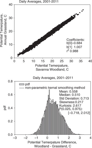
Fig. 3 (a) Seasonal course in diel-averaged potential temperature between an oak savanna and an annual grassland ecosystem. (b) Seasonal course in volumetric soil moisture. The data were bin-averaged by day for the period 2001–2011.

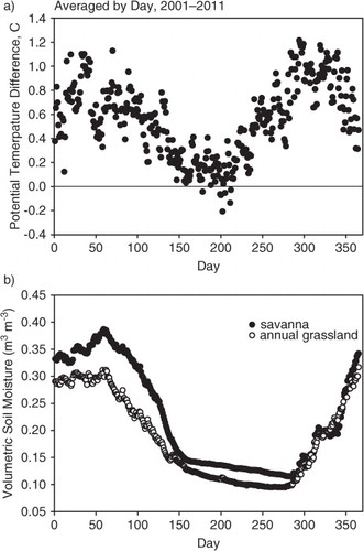
Fig. 4 Mean diurnal plot of air temperature over an oak savanna and an annual grassland. These data were binned by hour and were averaged over multiple years. (a) dormant period months, November–December–January, N–D–J; (b) summer (June–July–August, J–J–A).

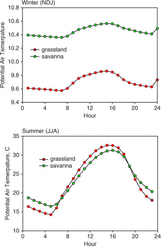
Fig. 5 Yearly course in daily-integrated net radiation flux density, averaged by day for the period 2001–2011, for a grassland and savanna ecosystem.

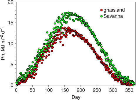
Table 1. Mean annual sums of energy flux densities and mean annual average of potential air temperatures

Variable	Unit	Annual grassland	Oak savanna
R net	GJ m^−2 y^−1	2.326	3.175
H	GJ m^−2 y^−1	1.574	1.993
LE	GJ m^−2 y^−1	0.844	1.260
G	GJ m^−2 y^−1	0.0393	0.0081
θ pot	°C	15.56	16.16

Table 2. Comparison in mean differences in daily-integrated energy fluxes and average potential temperature over an oak savanna and annual grassland

	Units	Mean difference: woodland – grass	95% CI
R net	MJ m^−2 d^−1	2.32	±0.122
H	MJ m^−2 d^−1	0.667	±0.050
λE	MJ m^−2 d^−1	0.6283	±0.046
θ pot	°C	0.558	±0.0228

Note: Statistics on the 95% confidence interval is given on 3770 degrees of freedom.

Fig. 6 (a) Yearly course in daily-integrated sensible heat flux density (H), averaged by day for the period 2001–2011, for a grassland and savanna ecosystem. (b) Yearly course in daily-integrated latent heat flux density (LE), averaged by day for the period 2001–2011, for a grassland and savanna ecosystem.

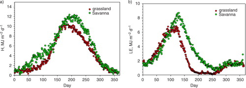
Fig. 7 Yearly course in the daily-average difference between the aerodynamic surface temperature, as computed from the surface energy balance, and air temperature.

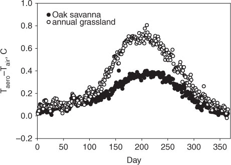
Fig. 8 (a) Yearly course in daily-averaged aerodynamic resistance (R _a), averaged by day for the period 2001–2011, for a grassland and savanna ecosystem. (b) Yearly course in daily-average surface resistance (R _sfc), averaged by day for the period 2001–2011, for a grassland and savanna ecosystem.

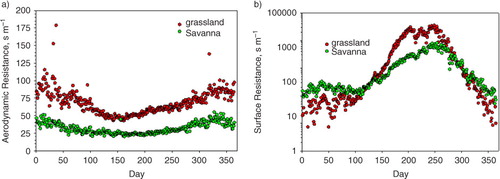
Fig. 9 Model computations of air temperature, referenced to temperatures above conditions experienced by the savanna (R _a=20 s m⁻¹; R _sfc=200 s m⁻¹; albedo=0.15), for summer-like weather. The model was run for a range of values in the aerodynamic and surface resistances. We assumed the albedo of the grass was 0.3.

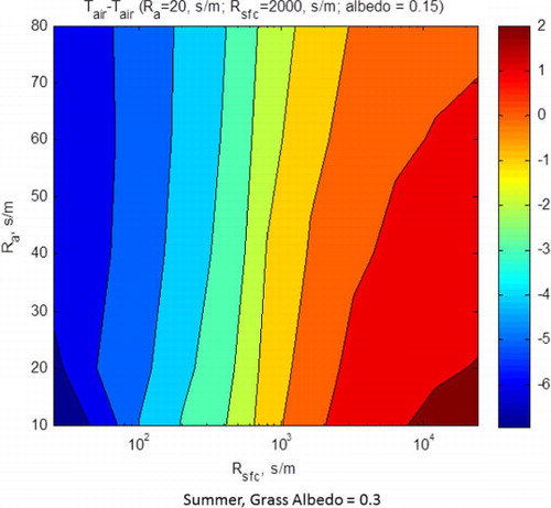
Fig. 10 (a) Model computations of air minus radiative surface temperatures, as a function of aerodynamic and surface resistances. (b) Model computations of net radiation, as a function of aerodynamic and surface resistances. Computations assumed albedo equalled 0.3 and summer time conditions of temperature and sunlight.

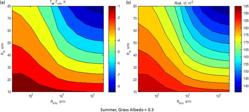
Fig. 11 Three-dimensional plot between maximum growth of the planetary boundary layer as a function of the aerodynamic and surface resistances. Computations were performed for summertime meteorological conditions and the biophysical conditions of the annual grass.

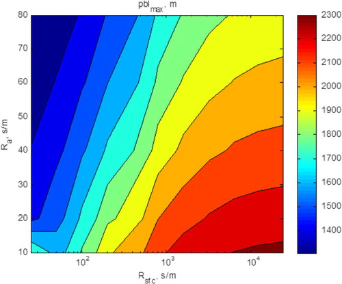
Fig. 12 Model computations of air temperature, referenced to temperatures above conditions experienced by the savanna (R _a=20 s m⁻¹; R _sfc=200 s m⁻¹; albedo=0.15), for winter-like meteorological conditions. The model was run for a range of values in the aerodynamic and surface resistances. We assumed the albedo of the grass was 0.15.

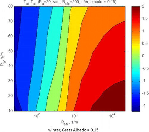
Fig. 13 Three-dimensional plot between maximum growth of the planetary boundary layer, shown as a function of the aerodynamic and surface resistances. Computations were performed for winter-time meteorological conditions and the biophysical conditions of the annual grass.

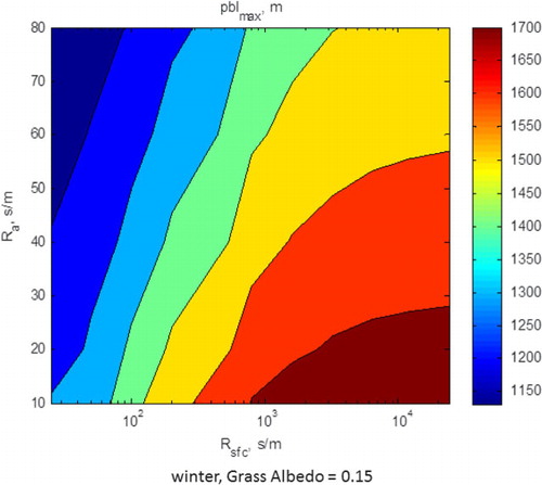
Table A1. List of initial conditions and parameter values used to evaluate the coupled surface energy balance/boundary layer model

	R gmax	Air temperature, t=0	Humidity	Albedo, grass	Albedo, savanna	R sfc, grass	R sfc, savanna
Summer	1000 W m^−2	20°C	1.5 kPa	0.20	0.15	25 s m^−1	200 s m^−1
Winter	500 W m^−2	10°C	1.0 kPa	0.40	0.15	10000 s m^−1	3000 s m^−1

R _gmax is the value of solar radiation at mid-day. R _sfc is the surface resistance.

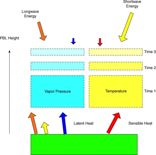
Fig. A1 Schematic of the coupled surface energy balance and planetary boundary layer model. The model identifies the energy fluxes at the lower and upper boundaries of the planetary boundary layer and how the layer grows with each time step.