Figures & data
Fig. 1 Computed climate response signals to greenhouse-gas emissions alone (G) and a combination of greenhouse-gas and sulphate aerosol emissions (GS), with associated 95% confidence ellipses, for climate simulations of the Hadley Centre, the Max Planck Institute for Meteorology and the Geophysical Fluid Dynamics Laboratory. Fingerprint patterns were computed using the climate models of MPIM (a) and the Hadley Centre (b). Most GS simulations lie within, most G simulations outside the relevant 95% confidence ellipses. Reproduced from Barnett et al. (Citation1999).
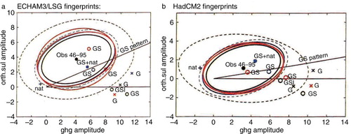
Fig. 2 Vertical profiles of temperature change for five different forcings and the resultant total force (f). The computed total change agrees well with observations. The decomposition confirms that most of the observed change is due to greenhouse-gas forcing – from Karl et al. (Citation2009).
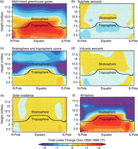
Fig. 3 Ten-year averages of the number of monthly-mean heat records at 17 stations worldwide (corresponding to a total of 17×12=204 heat records).
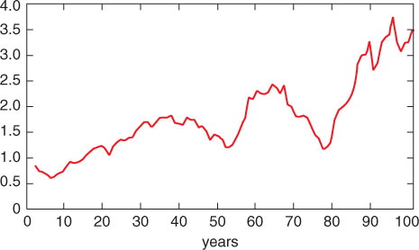
Fig. 4 Qualitative distribution of uncertainties associated with the detection, attribution, prediction and impact of climate change, with attendant widening risks.
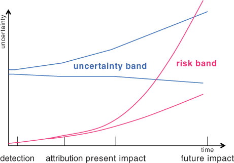
Fig. 5 Closing the wedge between a typical business-as-usual (BAU) greenhouse-gas emission path and a sustainability path that remains below the 2°C global warming guard rail. Renewable-energy technologies are ordered with respect to present costs. Solar energy is the largest, essentially unlimited, resource.
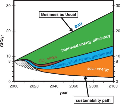
Fig. 6 Vensim-software sketch (cf. http://www.vensim.com) of the stocks (boxes) and flows (choke valves – or hour glasses) of a simple real-economy model (see text). Details of the actor-dependent variables controlling the stocks and flows are not shown.
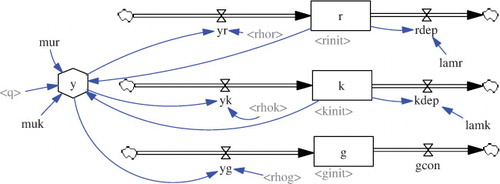
Fig. 7 Evolution of production-distribution factors for the simulations BAU (ρ r =0, ρ k =0.65, ρ g =0.35) and GREEN (green curve, with ρ g =0.35 and ρ r /ρ k monotonically increasing).
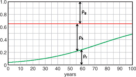
Fig. 8 Computed growth of GDP for a business-as-usual scenario (blue) and a reduced-emission scenario (green) for which the global warming remains below 2°C. (GDP is represented in arbitrary currency units ‘$’/year). Mitigation measures incur a growth delay over a period of 100 yr of only a few years.
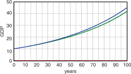
Fig. 9 Impact of the two scenarios BAU (blue) and GREEN (green) on global mean temperature (a) and welfare (b).
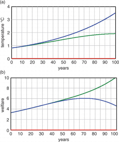
Fig. 10 Evolution of GDP (a) and welfare (b) for four BAU scenarios corresponding to ρ k =0.25, 0.35, 0.45, 0.55, with ρ r =0 in all cases. The reference scenario BAU (blue), with ρ k =0.35, yields the highest welfare values.
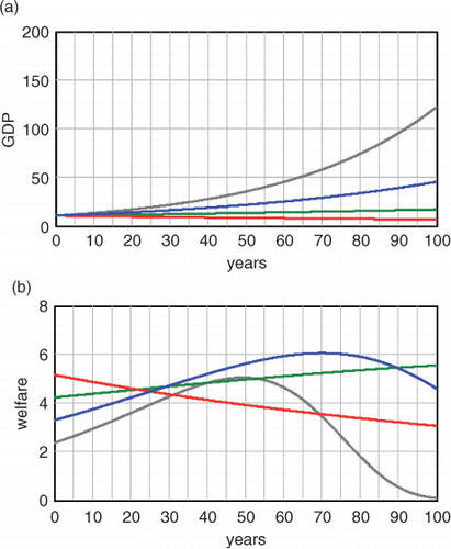
Fig. 11 Vensim-software sketch of the module representing the financial system coupled to the production module of . Money stocks and flows assigned to firms and investors are separated into renewable-energy-related liquidity and assets (left) and fossil-energy-related liquidity and assets (right). Details of the various inputs to the stocks and flows are not shown.
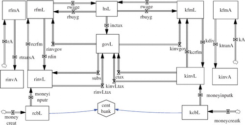
Table 1. Model runs of the coupled production-financial sectors, classed into supply-driven models S and supply-demand-feedback models F
Fig. 12 Alternative evolutions of the financial sector of the model MADIAMS for the same evolution BAU of the real-economy sector. The scenario BAL (blue) corresponds to balanced wealth growth of all economic actors commensurate with real economic growth, while the government-deficit scenario DEF (red) yields higher but non-sustainable values of household welfare and firm liquidity, at the cost of increasing government deficits.
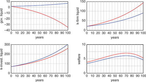
Fig. 13 Alternative predictions of the impact of strict saving measures to adjust the deficit-budget evolution path DEF (red curves) to the balanced-budget growth path BAL (green curves). The simulation SAV (blue curves) assumes a monotonic relaxation to the balanced-budget path, while the simulation REC (black curves) predicts a severe recession with major unemployment.
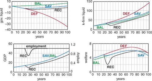
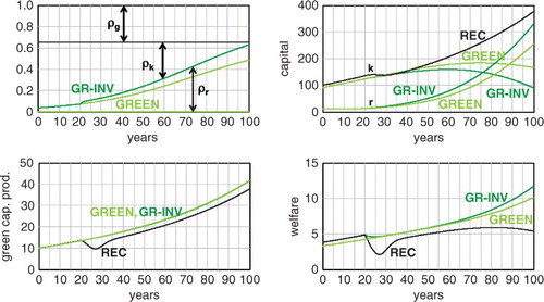
Fig. 14 Interrelation between decarbonisation and stabilisation of the financial markets. Simulation GR-INV (dark green curves) shows the impact of government savings measures accompanied by enhanced Keynesian investments in renewable energy. Simulation REC (black curves) shows the impact of savings measures alone, leading to a recession. Also shown is the original decoupled real-economy decarbonisation simulation GREEN (light green curves).