Figures & data
Fig. 1 Asian dust monitoring stations over Asian dust source regions operated by the Korea Meteorological Administration (KMA) since 2005 (○) and 2007 () and by the CMA (▵), Asian dust monitoring tower (▴), and four domestic observational sites operated by the KMA (▪). Only four representative observational sites in Korea are shown.
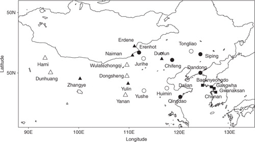
Fig. 2 The model domain for this study. The box over the Korean Peninsula denotes the area where a response function was defined.
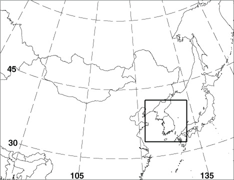
Table 1. Asian dust events that affected the Korean Peninsula from 2005 to 2010
Table 2. Ratio of linearly evolved perturbation to nonlinearly evolved perturbation in the projection area, averaged over all cases
Fig. 3 Monthly occurrence of Asian dust events affecting the Korean Peninsula from 2005 to 2010.
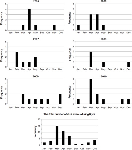
Table 3. Annual frequency distributions of the source regions of Asian dust events that affected the Korean Peninsula from 2005 to 2010
Table 4. Annual frequency distributions of Asian dust events that affected the Korean Peninsula from 2005 to 2010, categorized by the model integration time
Fig. 4 (a) The trajectories of all cases, (b) the representative trajectories of clustered groups using a regression analysis, and the trajectories of: (c) group 1, (d) group 2, (e) group 3, and (f) group 4.
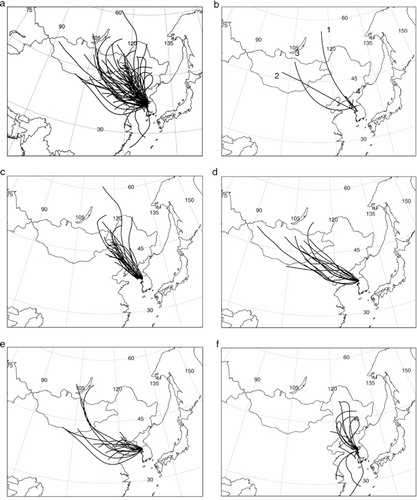
Fig. 5 The average surface-pressure patterns (black line) and 500 hPa geopotential height (blue line) at the occurrence times of maximum PM10 concentrations on the Korean Peninsula for: (a) group 1, (b) group 2, (c) group 3, and (d) group 4.
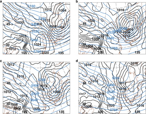
Table 5. Monthly frequency distributions of clustered groups of Asian dust events that affected the Korean Peninsula from 2005 to 2010
Table 6. Frequency distributions of clustered groups of Asian dust events that affected the Korean Peninsula from 2005 to 2010, categorized by the model integration time
Fig. 6 (a) Composite of the sensitivity field and (b) the sensitivity frequency field for all 46 cases, calculated using the energy forecast error as a response function for adjoint sensitivity calculation. (c) Composite of the sensitivity field and (d) the sensitivity frequency field for all 46 cases, calculated using the low-level pressure forecast error as a response function for adjoint sensitivity calculation.
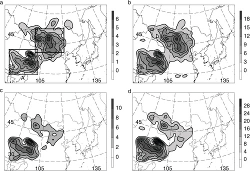
Fig. 7 Vertical profiles of the composite sensitivities (solid: total energy; dashed: kinetic energy; and dotted: potential energy) for boxes (a) A and (b) B in (a).
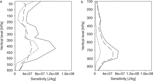
Fig. 8 The composite sensitivity frequency fields for the cases in (a) group 1, (b) group 2, (c) group 3, and (d) group 4.
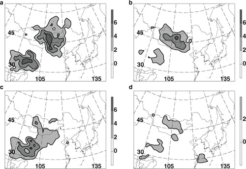
Fig. 9 The average surface-pressure patterns (black line) and 500 hPa geopotential height (blue line) at the initial time of the model integrations for: (a) group 1, (b) group 2, (c) group 3, and (d) group 4.
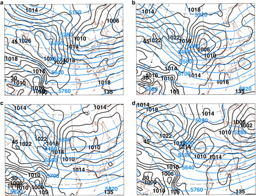
Fig. 10 The composite sensitivity frequency fields for the cases categorised by model integration times of: (a) 18–24 hours, (b) 30–36 hours, (c) 42–48 hours, and (d) 54–72 hours.
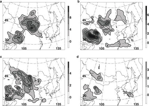
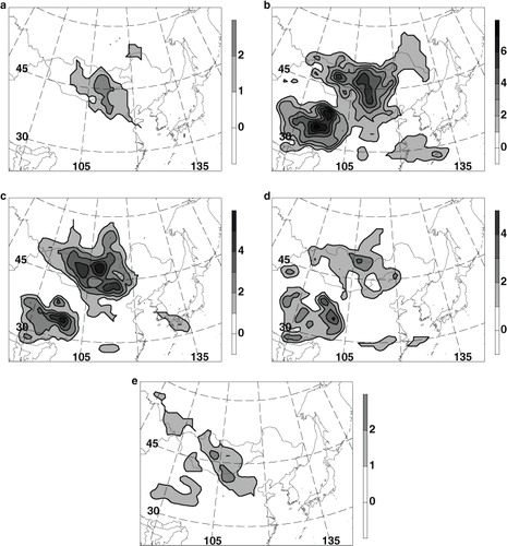
Fig. 11 The composite sensitivity frequency fields for the events that occurred in: (a) February, (b) March, (c) April, (d) May, and (e) December.