What controls precipitation δ¹⁸O in the southern Tibetan Plateau at seasonal and intra-seasonal scales? A case study at Lhasa and Nyalam

Figures & data

Fig. 1 2005–2007 averaged Outgoing Long Wave radiation (OLR, shading, downloaded from http://www.esrl.noaa.gov/psd/data/gridded/data.interp_OLR.html) showing convective activity as minima in OLR due to cold cloud tops and 500 hpa zonal wind speed (dashed contours) and wind vectors (arrows, downloaded from http://www.esrl.noaa.gov/psd/data). The zonal wind isolines highlight the Tibetan high-pressure system. The surface wind vectors clearly depict the Indian monsoon flow and the westerlies (a) in summer (JJAS) and (b) in winter (DJF).

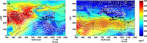
Table 1. Summary of precipitation data at Lhasa and Nyalam stations from 2005 to 2007

Station	Latitude	Longitude	Elevation	Period	n	T (°C)	P (mm)	Annual δ^18O (‰)
				2005 Jan 10–2005 Oct 29	130	11.55	475	−16.36
Lhasa	29° 42′ N	91° 08′ E	3658 m	2006 Mar 13–2006 Nov 4	95	12.25	322.5	−13.23
				2007 Feb 5–2007 Nov 6	69	12.58	470.6	−15.59
				2005 Jan 8–2005 Dec 24	72	3.02	468.1	−10.04
Nyalam	28° 11′ N	85° 58′ E	3810 m	2006 Jan 31–2006 Dec 13	134	5.96	669.5	−15.06
				2007 Feb 4–2007 Sep 28	111	6.89	499	−15.22

“n”=number of samples.

Note that no samples were obtained in August and September 2005 at Nyalam.

Fig. 2 Temporal variations of daily precipitation δ¹⁸O and local temperature, precipitation amount and OLR at Lhasa (a) and Nyalam (b) from 2005 to 2007. Seasonal patterns of monthly weighted precipitation δ¹⁸O, corresponding monthly mean temperature, precipitation amount and local OLR at Lhasa (c) and Nyalam (d) during 2005–2007. The black triangles highlight extreme events (identified from peak precipitation combined with depleted δ¹⁸O) at both stations on 16 August 2005, 17 August 2007, 24 September 2007, 2 July 2006 and 20 July 2007.

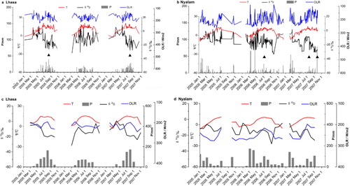
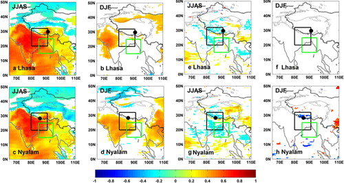
Fig. 3 Temporal correlations between daily precipitation δ¹⁸O at Lhasa (a) or at Nyalam (c) and precipitation amount in other grid points of the domain, in JJAS. (b) and (d): same as (a) and (c) but for DJF. (e) and (f): same as (a) and (c) but for monthly data. Temporal correlations between daily precipitation δ¹⁸O at Lhasa (g) or at Nyalam (h) and OLR in other grid points of the domain, in JJAS. On all maps, only correlations significant at the 95% confidence level are shown. The black rectangle shows the Zone 1 region discussed in the text.

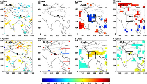
Fig. 4 Correlation coefficient (R) between the precipitation δ¹⁸O and local OLR averaged over J _m days (period prior to the event over which the convective activity is averaged) at Lhasa (a) and Nyalam (b). The numbers indicate the maximum values of J _m days for each period. (c) Correlation between the δ¹⁸O of events at Lhasa and the OLR averaged over the 13 d preceding each event in April, (d) 7 d preceding each event in May, (e) 3 d preceding each event in June–July, (i) 8 d preceding each event in August–September, and (j) 8 d preceding each event in JJAS. (k) No correlation can be calculated in DJF at Lhasa as only two events occurred. (f) Correlation between the δ¹⁸O of events at Nyalam and the OLR averaged over the 10 d preceding each event in April, (g) 16 d preceding each event in May, (h) 11 d preceding each event in June, (l) 19 d preceding each event in July–August, (m) 20 d preceding each event in JJAS and (n) 5 d preceding each event in DJF. The numbers in brackets indicate the number of events in different months. The black rectangle shows the Zone 1 region discussed in the text.

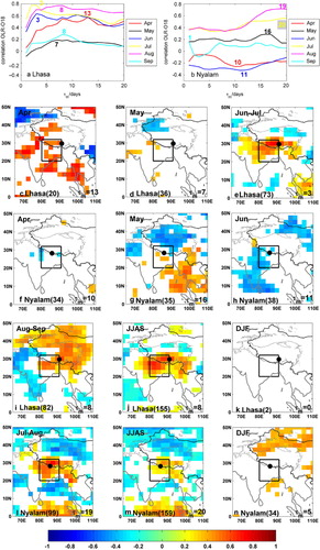
Fig. 5 (a–j) Back trajectories simulated by HYSPLT for Lhasa and Nyalam in different months (January, June, July, August and September). The percentage shows the frequency of each clustered back trajectory. Correlation coefficient (R) between the precipitation δ¹⁸O and OLR along the back trajectory averaged over J _m days (period prior to the event over which the convective activity is averaged) at Lhasa (k) and Nyalam (l). The numbers indicate the maximum values of J _m days for each period.

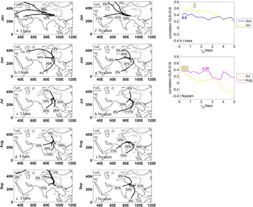
Fig. 6 Comparison of daily temperature from the zoomed LMDZiso simulations and observations at Lhasa (a) and Nyalam (d) during the observed period of 2005–2007; (b) and (e) same as (a) and (d) for precipitation amount; (c) and (f) same as (a) and (d) for precipitation δ¹⁸O. Relationships between precipitation amount and precipitation frequency at Lhasa (g) and Nyalam (h) from observations and zoomed LMDZiso simulations. The precipitation categories are calculated with steps of 2.5 mm, with events above 20 mm classified in one category.

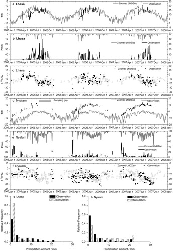
Fig. 7 Temporal correlation between temperature and precipitation δ¹⁸O at Lhasa (a) and Nyalam (c) from zoomed LMDZiso simulations in summer (JJAS); (b) and (d) same as (a) and (c) for winter (DJF); (e) and (g) same as (a) and (c) for precipitation amount; (f) and (h) same as (e) and (g) for winter (DJF). The black rectangle shows the Zone 1, and the green rectangle shows the Zone 2.