Determination of a lower bound on Earth's climate sensitivity

Figures & data

Fig. 1 GHG forcing as presented by the Goddard Institute for Space Studies (GISS; http://data.giss.nasa.gov/modelforce/RadF.txt), National Oceanic and Atmospheric Administration (NOAA; http://www.esrl.noaa.gov/gmd/aggi/AGGI_Table.csv) and the Representative Concentration Pathways group (RCP; http://www.pik-potsdam.de/~mmalte/rcps/data/20THCENTURY_MIDYEAR_RADFORCING.xls). All forcings are set equal at 1982 to permit comparison.

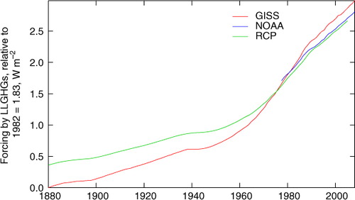
Fig. 2 Correlation of global temperature and GHG forcing. Temperature anomaly data are HadCrut3 (Brohan et al., 2006, as extended at http://www.cru.uea.ac.uk/cru/data/temperature/). Forcing (blend of RCP and NOAA as discussed in the text) is relative to preindustrial. Ratio of scales of two vertical axes was set by slope of graph of ΔT _s vs. forcing.

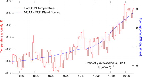
Fig. 3 Forcing by LLGHGs and non-LLGHG forcing over the time period 1970–2010 as given by the GISS and blended RCP-NOAA data sets.

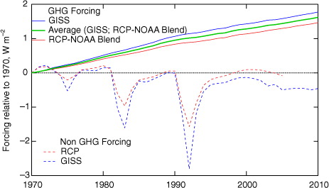
Fig. 4 Graph of temperature anomaly vs. forcing by LLGHGs for the years 1970–2010 (indicated by colour). Forcing is the average of GISS and blended RCP-NOAA, relative to 1970, Fig. 3. Slope S _tr=0.39±0.03 K/(W m⁻²), where the 1−σ uncertainty is based only on the uncertainty in the fit; forcing is relative to 1970; temperature anomaly HadCrut3 is relative to base period 1961–1990. Correlation coefficient r ²=0.80.

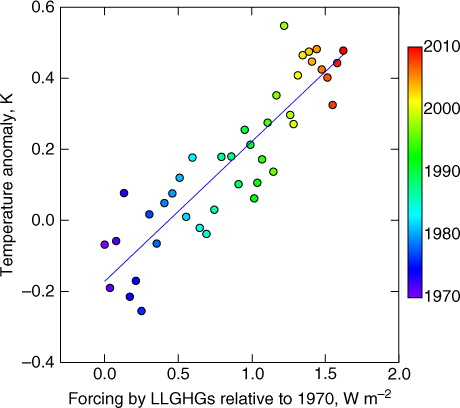
Table 1. Calculation of lower-bound transient and equilibrium sensitivities

Quantity	Unit	Best estimate	1−σ uncertainty	Lower 5% bound
ΔF (1970–2010)	W m^−2	1.465	0.234
S tr	K (W m^−2)^−1	0.394	0.071	0.278
S tr	K (3.7 W m^−2)^−1	1.460	0.262	1.031
N	W m^−2	0.374	0.032
ΔT s (1900–1990)	K	0.529	0.100
S eq	K (W m^−2)^−1	0.545	0.142	0.312
S eq	K (3.7 W m^−2)^−1	2.023	0.528	1.157

LLGHG forcing over period 1970–2010 ΔF is based on the mean of GISS and blended RCP-NOAA forcing data sets; uncertainty in forcing is taken as ±16% as discussed in text. Column 3 presents values for forcing by LLGHGs only and thus yields a best estimate for lower-bound transient and equilibrium sensitivity. Uncertainty in S _tr reflects uncertainties in ΔF and dΔT _s/dΔF. Heating rate N and associated uncertainty are from Table 2. Time range for ΔT _s is for middle of time period examined relative to assumed steady state at beginning of twentieth century. Last column shows lower bounds of the 5–95% uncertainty range, evaluated as the best-estimate value of the lower bound minus 1.64 times the 1−σ uncertainty for the probability distribution function for the quantity taken as normally distributed. Values of S _tr and S _eq expressed in the unit K (3.7 W m⁻²)⁻¹ are shown to permit comparison with commonly reported CO₂ doubling temperature ΔT _2×.

Fig. 5 Heat content of the world ocean to depth of 2000 m. Slope (0.48±0.02×10²² J yr⁻¹) of linear fit (blue) to data for years 1970–2008, indicated by arrows, corresponds to heating rate relative to the area of the planet N=0.30±0.01 W m⁻². Data from Levitus et al. (2012).

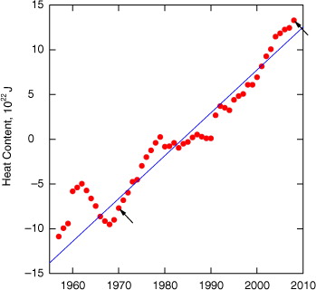
Table 2. Contributions to planetary heating rate

Component	Heating rate (W m^−2)	Uncertainty (W m^−2)	Start year	End year
Atmosphere	0.0057	0.0003	1980	2007
Land	0.0187	0.0006	1980	2006
Sea ice melt	0.0072	0.0005	1981	2007
Ice shelf melt	0.0022	0.00003	1982	2007
Ice sheet melt Greenland, Antarctica	0.0049	0.0002	1982	2006
Glaciers, small ice caps	0.0077	0.0002	1982	2007
Total non-ocean	0.0464	0.0009
Ocean to 2000 m	0.298	0.012	1970	2008
Ocean below 2000 m	0.030	0.030	1970	2008
Total ocean	0.327	0.032	1970	2008
Total	0.374	0.032

Non-ocean components of Earth's energy imbalance are based on Hansen et al. (2011). The rate of ocean heating, from Fig. 5, is based on Levitus et al. (2012).

Brohan P , Kennedy J. J , Harris I , Tett S. F. B , Jones P. D . Uncertainty estimates in regional and global observed temperature changes: a new data set from 1850. J. Geophys. Res. 2006; 111: D12106.

 Web of Science ®Google Scholar

Levitus S , Antonov J. I , Boyer T. P , Baranova O. K , Garcia H. E , co-authors . World ocean heat content and thermosteric sea level change (0–2000 m), 1955–2010. Geophys. Res. Lett. 2012; 39: L10603.

 Web of Science ®Google Scholar

Hansen J , Sato M , Kharecha P , von Schuckmann K . Earth's energy imbalance and implications. Atmos. Chem. Phys. 2011; 11: 13421–13449.

 Web of Science ®Google Scholar