Influence of coastal upwelling on the air–sea gas exchange of CO₂ in a Baltic Sea Basin

Figures & data

Fig. 1 Map of the Baltic Sea and Östergarnsholm site showing the position of the meteorological tower, the SAMI-sensor, and the Wave rider buoy (from Rutgersson et al., 2008).

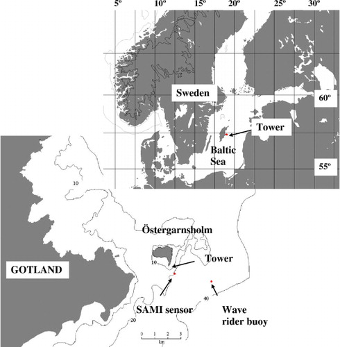
Fig. 2 Measurements at the Östergarnsholm site during Period 1: (a) wind direction (°); (b) wind speed (m s⁻¹); (c) air temperature (black solid line), water temperature from the SAMI sensor (grey solid line) and the wave rider buoy (grey dashed line) (°C); (d) pCO₂ in air (black solid line) and in water from the SAMI sensor (grey solid line) (µatm). The grey shaded area in (a) shows the wind direction 195°–225°, that is, the orientation of the southeastern part of the Gotland coastline.

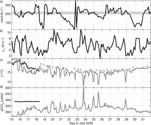
Fig. 3 Daily averaged satellite images of sea-surface temperature (SST) (°C) around the island of Gotland in the Baltic Sea during 14–22 July 2005 (Period 1). The colours represent the SST value described by the colour bar.

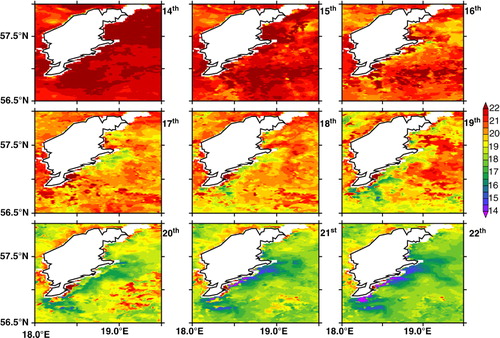
Fig. 4 Daily spatial standard deviation of sea-surface temperature (SST) (°C) in the area surrounding Gotland during 14–22 July 2005 (Period 1).

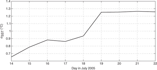
Fig. 5 Measurements at the Östergarnsholm site during part of Period 4: (a) wind direction (°); (b) wind speed (m s⁻¹); (c) air temperature at two levels (black solid line represents 10 m height and black dashed line at 26 m height), and water temperature from the SAMI sensor (grey solid line) (°C); (c) pCO₂ in air (black solid line) and in water from the SAMI sensor (grey solid line) (µatm).

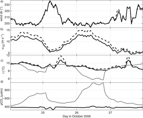
Fig. 6 As Fig. 3, but during the time period 24–29 October 2008 (Period 4).

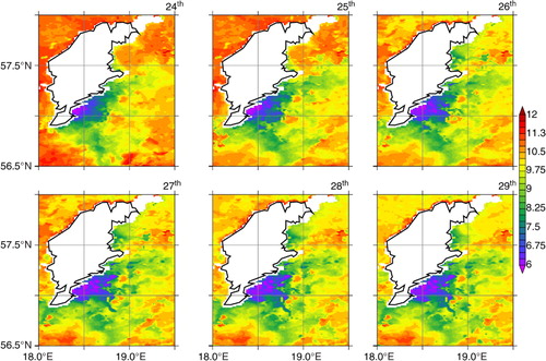
Fig. 7 (a) Fluxes of CO₂ (µmol m⁻² s⁻¹) and (b) air–sea transfer velocity (cm h⁻¹) during Period 1. Open circles represent in (a) fluxes estimated using the eddy-covariance method, (b) the transfer velocity calculated using eq. (1) and the measured fluxes. Filled circles represent in (a) calculated fluxes using eq. (1) and eq. (2) for the transfer velocity, (b) the transfer velocity according to eq. (2).

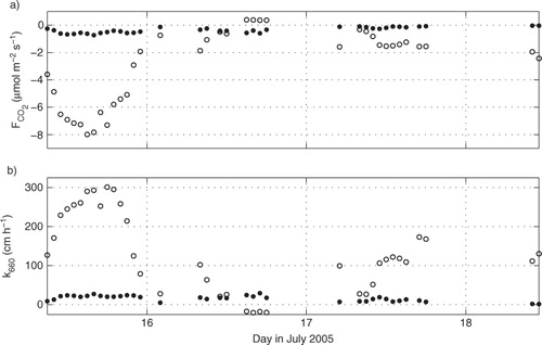
Fig. 8 (a) Fluxes of CO₂ (µmol m⁻² s⁻¹) and (b) air–sea transfer velocity (cm h⁻¹) during Period 4. Open circles represent in (a) fluxes at 10 m estimated using the eddy-covariance method, (b) the transfer velocity calculated using eq. (1) and the measured fluxes at 10 m. Crosses represent in (a) fluxes at 26 m estimated using the eddy-covariance method, (b) the transfer velocity calculated using eq. (1) and the measured fluxes at 26 m. Filled circles represent in (a) calculated fluxes using eq. (1) and eq. (2) for the transfer velocity, (b) the transfer velocity according to eq. (2).

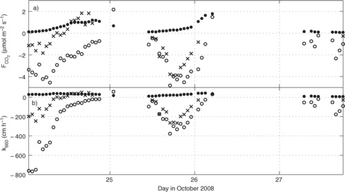
Fig. 9 The relation between pCO_2w (µatm) and sea-surface temperature (SST) (°C) (hourly average values) during Period 1 (dots). The crosses represent measurements during 2 d before the upwelling started.

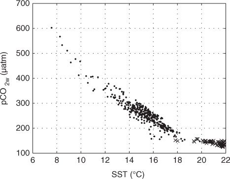
Fig. 10 The relation between pCO_2w (µatm) and sea-surface temperature (SST) (°C) (hourly average values) measured by the SAMI sensor. Black dots represent Period 1, grey dots Period 2, grey circles Period 3 and black circles represent Period 4. The lines represent the fitted linear relation between SST and pCO_2w.

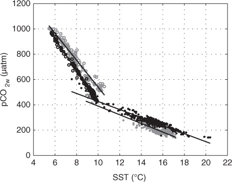
Table 1. Coefficients a and b in the linear relation between SST and pCO_2w, pCO_2w=a+b·SST, during the four upwelling periods

Period	a	B	r
1	−32	747	−0.94
2	−34	732	−0.91
3	−107	1604	−0.97
4	−125	1674	−0.99

Also presented is the correlation coefficient, r, between SST and pCO_2w.

Fig. 11 Water profiles of: (a) temperature (°C); (b) C_T (µmol kg⁻¹) for the Eastern Gotland basin estimated with a one-dimensional biogeochemical Baltic Sea model (Omstedt et al., 2009). The solid line refers to an average of July months during the years 2000–2009, and the dashed line refers to an average of October months during the same period.

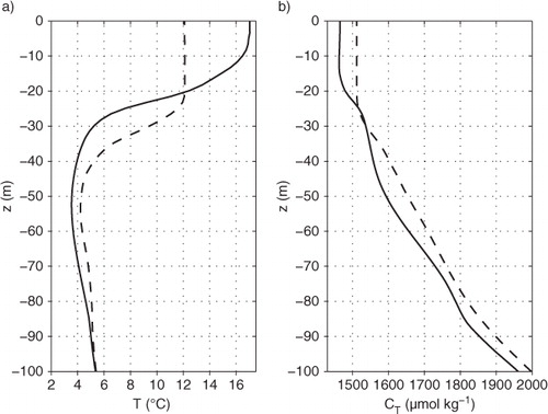
Fig. 12 The coloured area shows estimated fluxes (µmol m² s⁻¹) where upwelling is detected during Period 1 (19–24 July 2005) using the algorithm described in Section 2.2.1. The fluxes are estimated using the satellite sea-surface temperature (SST) and the SST–pCO_2w relation in Table 1, magnitude indicated by the colour bar.

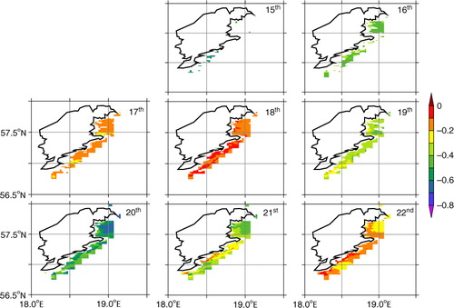
Fig. 13 As Fig. 12, but during the time period 24–27 October 2008. Notice the difference in scale from Fig. 12.

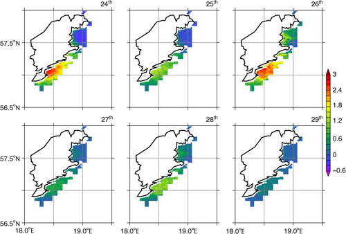
Fig. 14 Daily averaged sea-surface temperature (SST) (°C) and pCO_2w (µatm) during 14 July–3 August 2005 (Period 1). The solid lines are measured values showing upwelling with decreasing SST and increasing pCO_2w. The dashed lines illustrate interpolated values assuming no upwelling occurred during this period.

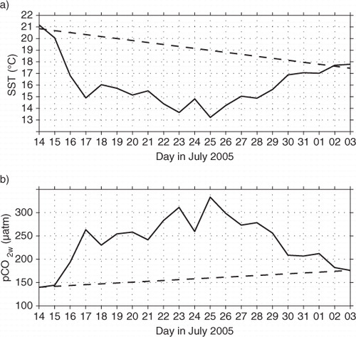
Table 2. The uptake/release of CO₂ (Gg) calculated without (A) and with (B) upwelling during the four upwelling events in the upwelling area off the south east coast of Gotland

Period	A	B	AD	ARD
1	−25.5	−20.5	5.0	19
2	−9.2	−3.8	5.4	59
3	+7.3	+22.7	15.4	211
4	+9.4	+32.8	23.4	250

Also presented are the absolute difference (AD) (Gg), and the absolute relative difference (ARD) (%), of the uptake/release with and without upwelling.

Rutgersson A , Norman M , Schneider B , Pettersson H , Sahlée E . The annual cycle of carbon dioxide and parameters influencing the air–sea carbon exchange in the Baltic Proper. J. Mar. Syst. 2008; 74: 381–394.

 Web of Science ®Google Scholar

Omstedt A , Gustavsson E , Wesslander K . Modelling the uptake and release of carbon dioxide in the Baltic Sea surface water. Continental. Shelf Res. 2009; 29: 870–885.

 Web of Science ®Google Scholar