Evaluating aerosol direct radiative effects on global terrestrial ecosystem carbon dynamics from 2003 to 2010

Figures & data

Fig. 1 Global potential natural vegetation map used in this study. The map shown here is the map of the dominant plant functional types in each 1°×1° grid cell. The labels are: (1) ice; (2) Alpine tundra and polar deserts; (3) wet tundra; (4) boreal forest; (5) temperate coniferous forest; (6) temperate deciduous forest; (7) grasslands; (8) xeric shrublands; (9) tropical forests; (10) xeric woodland; (11) temperate broadleaved evergreen forest; (12) Mediterranean shrublands.

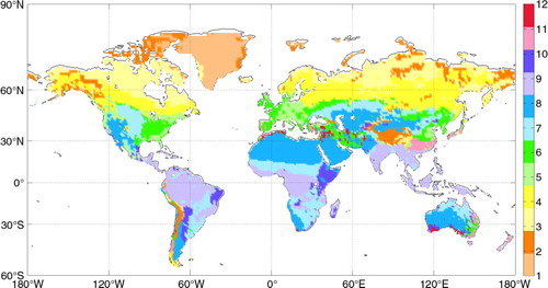
Table 1. MODIS parameters used in the calculation of downward solar radiation

Data fields	MODIS product name	Descriptions
Total_Ozone_Mean	MOD08_D3/ MYD08_D3	Total ozone column (cm)
Cloud_Top_Pressure_Mean	MOD08_D3/ MYD08_D3	Cloud top pressure (Pa)
Cloud_Optical_Thickness_Combined_Mean	MOD08_D3/ MYD08_D3	Cloud optical thickness
Angstrom_Exponent_Land_Mean	MOD08_D3/ MYD08_D3	Ångström exponent (Land) for 0.47 and 0.66 microns
Deep_Blue_Angstrom_Exponent_Land_Mean	MOD08_D3/ MYD08_D3	Deep Blue Ångström Exponent for land (0.412–0.47 micron)
Angstrom_Exponent_1_Ocean_Mean	MOD08_D3/ MYD08_D3	Ångström Exponent (0.550 and 0.865 micron) best solution
Optical_Depth_Land_And_Ocean_Mean	MOD08_D3/ MYD08_D3	Aerosol Optical Thickness at 0.55 microns for both Ocean and Land
Deep_Blue_Aerosol_Optical_Depth_550_Land_Mean	MOD08_D3/ MYD08_D3	Deep blue aerosol optical depth at 0.55 microns for land
Atmospheric_Water_Vapor_Mean	MOD08_D3/ MYD08_D3	Total perceptible water vapour column (cm)
Cloud_Fraction_Mean	MOD08_D3/ MYD08_D3	Cloud fraction
Albedo_WSA_vis Albedo_WSA_nir	MCD43C3	White-Sky land Albedo for the VIS and NIR broadbands

Fig. 2 Annual mean land surface solar radiation of 2003–2010 estimated with or without aerosols and their differences. The difference is calculated as the estimates with aerosols subtract the estimates without aerosols.

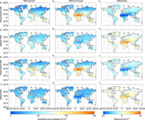
Fig. 3 Gap-filled 2003–2010 mean values of MODIS AOD, COD and cloud fraction over the global land area.

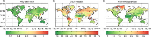
Fig. 4 Annually averaged differences of S0 and S1 carbon fluxes and land surface environmental variables over the period of 2003–2010. T_S is the land surface temperature; ST1 and SM1 are the first soil layer temperature and volumetric moisture content, respectively.

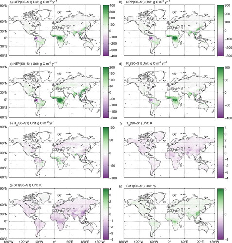
Fig. 5 Differences of the continent-based carbon fluxes over the study period. Error bars denote the standard deviation for the 8-yr values.

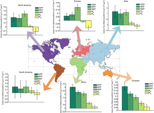
Fig. 6 Aerosol-caused changes of annual average global leaf area index.

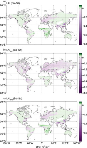
Fig. 7 Aerosol-induced changes of carbon fluxes and environmental variables at different leaf area index levels. The change is the difference between annual mean values of these variables of the S0 and S1 estimates.

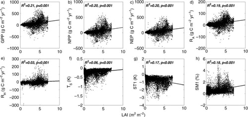
Fig. 8 Differences of plant functional type based carbon fluxes and environmental conditions over the study period. Error bars represent the standard deviation for the 8-yr values. T_S is the land surface temperature; ST1 and SM1 are the first soil layer temperature and volumetric moisture content, respectively.

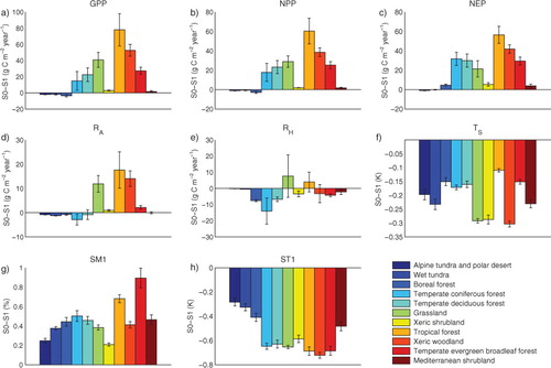
Fig. 9 Annual average leaf area index for each plant functional type of the S0 simulation. Error bars represent the standard deviation for the 8-yr values.

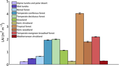
Fig. 10 Photosynthetic parameters for sunlit and shaded leaves. J_C and J_E: the leaf-scale Rubisco-limited photosynthesis rate and light-limited photosynthesis rate (Units: µmol CO₂ m⁻² s⁻¹), respectively; GPP_sun and GPP_sha: canopy GPP (photosynthesis) for sunlit and shaded leaves (Units: g C m⁻² yr⁻¹), respectively; T_l: annual average leaf temperature (Units: K).

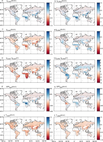
Fig. 11 Scatterplots of aerosol-induced changes of key carbon fluxes (GPP and R_H) and environmental conditions (T_S, ST1 and SM1). Units for the carbon fluxes are g C m⁻² yr⁻¹.

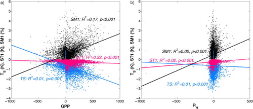
Fig. 12 Sensitivity of monthly averaged key carbon fluxes (GPP and RH) to unit change of AOD at different thermal and humid conditions. The units of the sensitivity of both the scatterplot and bar plots are g C mon⁻¹.

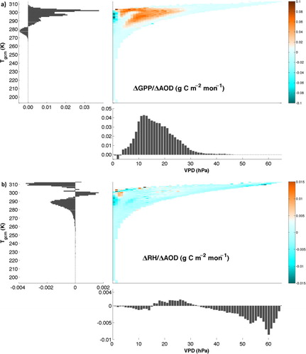
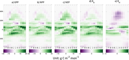
Fig. 13 Zonal mean differences between carbon fluxes (calculated as S0–S1) averaged over the study period.