Close relationship between spectral vegetation indices and V_cmax in deciduous and mixed forests

Figures & data

Table 1. Site description including name and location (latitude and longitude), canopy height, duration of measurements, stand age, dominant species composition, and references for each flux site in this study

Site	Country	Latitude, longitude	Canopy height (m)	Time span	Stand age (years)	Dominant species composition	References
CBS	China	42°24′9″N, 128°05′45″E	26	2003–2005	200	Pinus koraiensis, Tilia amurensis, Acer mono, Fraxinus mandshurica, Quercus mongolica	Yu et al., 2008; Zhang et al., 2009
SKOA	Canada	53°37′12″N, 106°11′24″W	23	2000–2002	74	Trembling aspen, Populus tremuloides Michx.	Gower et al., 1997; Krishnan et al., 2006; Mo et al., 2008
UMBS	America	45°33′35″N, 84°42′50″W	22	2000–2002	90	Populus grandidentata Michx., Quercus rubra L. Fagus grandifolia Ehrh., Acer rubrum L. and Pinus strobus L.	Curtis et al., 2005; Gough et al., 2013

Table 2. Standard deviations and ranges of model parameters optimised

Symbol	Unit	Standard deviation	Range
Vcmax	µmol m^−2 s^−1	4	8–60
M	Dimensionless	0.8	2–16
D0	kPa	0.15	1.1–2.2

Fig. 1 The seasonal variations in 8 d average air temperature, T_a (a–c), cumulative 8 d solar radiation, S_w (d–f), and 8 d average vapour pressure deficit, VPD (g–i), for CBS, SKOA and UMBS.

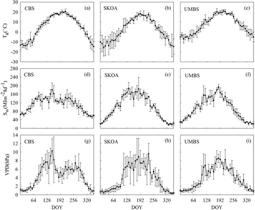
Fig. 2 Monthly cumulative precipitation, PPT: at (a) CBS, (b) SKOA and (c) UMBS.

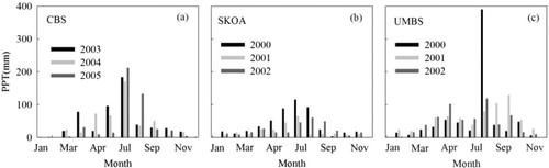
Fig. 3 Seasonal changes in NDVI, EVI and V_cmax: (a–c) for CBS during 2003–2005; (d–f) for SKOA during 2000–2002; and (g–i) for UMBS during 2000–2002.

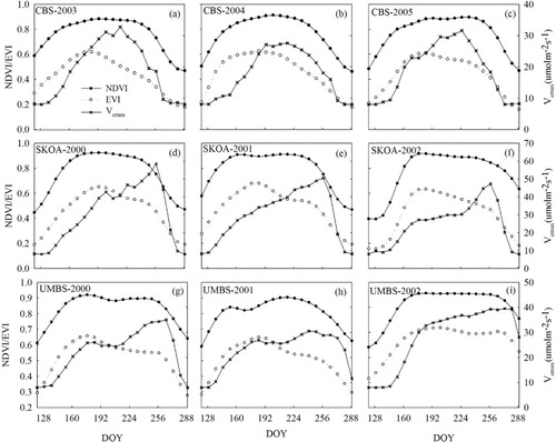
Fig. 4 Ensemble daily (24 h) GPP, SH and LE fluxes, and observations: (aa–ai) at CBS during 2003–2005; (ba–bi) at SKOA during 2000–2002; and (ca–ci) at UMBS during 2000–2002. The black and grey dots showed predicted and observed GPP, SH and LE, respectively.

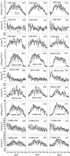
Table 3. Statistics of the linear regression (Y=aX+b) between observed (as Y) and simulated (as X) daily fluxes of GPP (g C m⁻² d⁻¹), LE (W m⁻²) and SH (W m⁻²)

			Parameters optimised using EnKF
Site	ITEM	Year	a	b	R^2	RMSE
CBS	GPP	2003	0.85	1.00	0.89	3.09
		2004	0.89	0.92	0.90	2.99
		2005	0.87	1.14	0.87	2.99
	SH	2003	1.11	−2.61	0.79	25.13
		2004	1.01	−1.49	0.79	24.46
		2005	0.89	4.64	0.79	24.60
	LE	2003	0.91	5.99	0.87	28.92
		2004	0.92	7.63	0.80	26.15
		2005	0.89	7.99	0.79	24.68
SKOA	GPP	2000	0.80	0.56	0.91	4.08
		2001	0.82	1.00	0.91	4.03
		2002	0.92	0.46	0.89	3.52
	SH	2000	0.81	2.28	0.78	37.14
		2001	0.92	−1.76	0.78	28.92
		2002	0.89	−3.19	0.79	47.43
	LE	2000	0.93	3.92	0.81	36.41
		2001	1.04	4.21	0.80	37.65
		2002	1.01	3.25	0.81	29.09
UMBS	GPP	2000	0.86	1.24	0.86	3.11
		2001	0.82	0.62	0.85	3.10
		2002	0.85	0.11	0.93	3.95
	SH	2000	1.05	−18.96	0.90	45.24
		2001	0.85	−10.54	0.80	35.81
		2002	0.93	−9.29	0.82	40.28
	LE	2000	0.88	−1.09	0.79	33.63
		2001	0.81	−5.54	0.82	35.28
		2002	0.86	−6.44	0.85	43.65

Fig. 5 Relationships between (aa–ai) NDVI and (ba–bi) EVI and V_cmax over the growing seasons from DOY 121–289 during 2003–2005 at CBS. Data were divided into two phenological phases: first phase (solid circles) and second phase (open circles).

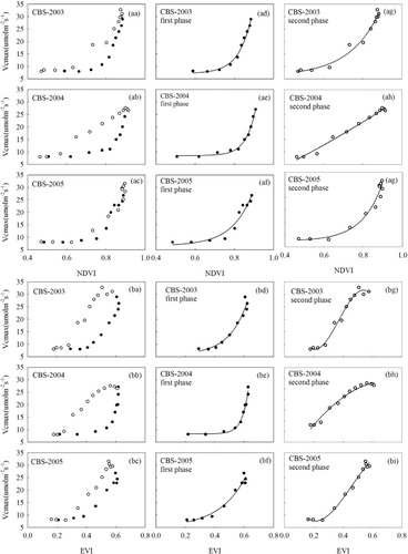
Fig. 6 Relationships between (aa–ai) NDVI and (ba–bi) EVI and V_cmax over the growing seasons from DOY 121–289 during 2000–2002 at SKOA. Data were divided into two phenological phases: first phase (solid circles) and second phase (open circles).

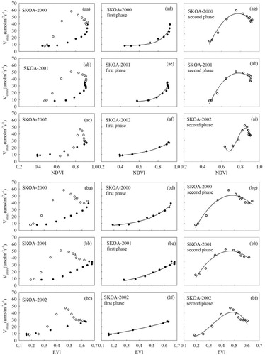
Fig. 7 Relationships between (aa–ai) NDVI and (ba–bi) EVI and V_cmax over the growing seasons from DOY 121–289 during 2000–2002 at UMBS. Data were divided into two phenological phases: first phase (solid circles) and second phase (open circles).

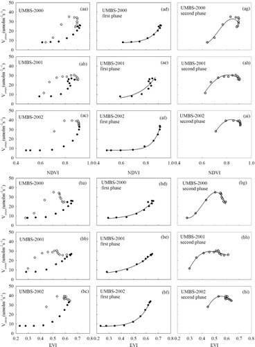
Table 4. Regression results of V_cmax (y, µmol m⁻²s⁻¹) with vegetation indices (NDVI and EVI). Only the best regression models are shown, and the highest R² and significance level are indicated

Site	VIs	Phase	Regression equation	R^2	p
CBS	NDVI	First-2003	y=7.18+3.0781E−005exp(15.23x)	0.99	p<0.001
		Second-2003	y=6.20+0.08exp(6.52x)	0.98	p<0.001
		First-2004	y=8.52+2.5761E−007exp(19.94x)	0.99	p<0.001
		Second-2004	y=−9.57+30.36x+11.37x^2	0.99	p<0.001
		First-2005	y=6.65+0.004exp(9.66x)	0.94	p<0.001
		Second-2005	y=7.40+0.005exp(9.53x)	0.96	p<0.001
	EVI	First-2003	y=5.73+0.14exp(8.10x)	0.95	p<0.001
		Second-2003	y=47.34−438.12x+1468.61x^2−1316.60x^3	0.98	p<0.001
		First-2004	y=8.30+1.0102E−005exp(22.90x)	0.98	p<0.001
		Second-2004	y=13.42−111.80x+530.35x^2−510.84x^3	0.99	p<0.001
		First-2005	y=5.05+0.68exp(5.56x)	0.97	p<0.001
		Second-2005	y=27.55−210.00x+647.11x^2−472.75x^3	0.99	p<0.001
SKOA	NDVI	First-2000	y=8.45+0.002exp(10.25x)	0.95	p<0.001
		Second-2000	y=−277.84+855.21x−552.33x^2	0.96	p<0.001
		First-2001	y=6.52+0.003exp(10.06x)	0.88	p<0.001
		Second-2001	y=−234.28+724.57x−463.69x^2	0.96	p<0.001
		First-2002	y=5.22+0.88exp(3.51x)	0.99	p<0.001
		Second-2002	y=7207.25+7207.25x+38384.699x^2−16744.62x^3	0.96	p<0.001
	EVI	First-2000	y=4.37+1.13exp(5.17x)	0.99	p<0.001
		Second-2000	y=−77.65+530.93x−547.28x^2	0.94	p<0.001
		First-2001	y=−4.86+5.06exp(2.99x)	0.97	p<0.001
		Second-2001	y=−79.73+541.62x−575.89x^2	0.95	p<0.001
		First-2002	y=−16.85+21.22exp(1.17x)	0.99	p<0.001
		Second-2002	y=45.32−531.36x+2127.73x^2+2163.54x^3	0.88	p<0.001
UMBS	NDVI	First-2000	y=7.34+0.0002exp(12.62x)	0.98	p<0.001
		Second-2000	y=1537.02−6582.46x+9256.88x^2−4229.02x^3	0.80	p<0.005
		First-2001	y=3.69+0.03exp(7.73x)	0.80	p<0.001
		Second-2001	y=−306.67+830.96x−511.65x^2	0.93	p<0.001
		First-2002	y=8.141+5.2163E−006exp(16.80x)	0.99	p<0.001
		Second-2002	y=−505.51+1303.61x−777.90x^2	0.89	p<0.001
	EVI	First-2000	y=6.39+0.09exp(8.19x)	0.95	p<0.001
		Second-2000	y=251.32−2086.41x+5672.25x^2−4730.79x^3	0.97	p<0.001
		First-2001	y=4.26+0.57exp(5.71x)	0.99	p<0.001
		Second-2001	y=−190.30+1223.58x−2216.50x^2+1296.40x^3	0.96	p<0.001
		First-2002	y=7.16+0.02exp(11.48x)	0.99	p<0.001
		Second-2002	y=−492.03+2341.052x−3581.89x^2+1669.97x^3	0.90	p<0.001

Yu G.-R. , Zhang L.-M. , Sun X.-M. , Fu Y.-L. , Wen X.-F. , co-authors . Environmental controls over carbon exchange of three forest ecosystems in eastern China. Global Change Biol. 2008; 14: 2555–2571.

 Web of Science ®Google Scholar

Zhang J. , Hu Y. , Xiao X. , Chen P. , Han S. , co-authors . Satellite-based estimation of evapotranspiration of an old-growth temperate mixed forest. Agr. Forest Meteorol. 2009; 149: 976–984.

 Web of Science ®Google Scholar

Gower S. T. , Vogel J. G. , Norman J. M. , Kucharik C. J. , Steele S. J. , co-authors . Carbon distribution and aboveground net primary production in aspen, jack pine, and black spruce stands in Saskatchewan and Manitoba, Canada. J. Geophys. Res. Atmos. 1997; 102: 29029–29041.

 Web of Science ®Google Scholar

Krishnan P. , Black T. A. , Grant N. J. , Barr A. G. , Hogg E. H. , co-authors . Impact of changing soil moisture distribution on net ecosystem productivity of a boreal aspen forest during and following drought. Agr. Forest Meteorol. 2006; 139: 208–223.

 Web of Science ®Google Scholar

Mo X. , Chen J. M. , Ju W. , Black T. A . Optimization of ecosystem model parameters through assimilating eddy covariance flux data with an ensemble Kalman filter. Ecol. Model. 2008; 217: 157–173.

 Web of Science ®Google Scholar

Curtis P. S. , Vogel C. S. , Gough C. M. , Schmid H. P. , Su H. B. , co-authors . Respiratory carbon losses and the carbon-use efficiency of a northern hardwood forest, 1999–2003. New Phytol. 2005; 167: 437–455.

 Google Scholar

Gough C. M. , Hardiman B. S. , Nave L. E. , Bohrer G. , Maurer K. D. , co-authors . Sustained carbon uptake and storage following moderate disturbance in a Great Lakes forest. Ecol. Appl. 2013; 23: 1202–1215.

 Google Scholar