Decadal variability of clouds, solar radiation and temperature at a high-latitude coastal site in Norway

Figures & data

Fig. 1 Difference between the monthly averaged global irradiance and the sum of diffuse and direct irradiance, measured at the Florida site in Bergen, Norway, from 1991 to 2013, shown as a time series (left panel) and a histogram (right panel).

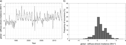
Fig. 2 Comparison of the distribution of (a) cloud cover and (b) cloud base observations at the Florida and Flesland stations in Bergen, Norway. The observational stations are presented in Section 2 and the cloud data are discussed in Section 3.2.

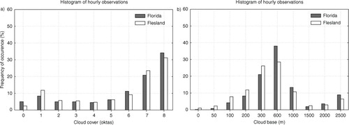
Fig. 3 Time series of temperature measured at the Florida (solid line), Flesland (dotted line) and Fredriksberg (dashed line) sites in Bergen. The thinner lines show the annual mean time series while the thicker lines are smoothed time series of the observational time series (shown only for the Florida site).

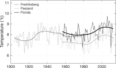
Fig. 4 Time series of the (a) global irradiance, (b) sunshine duration, (c) atmospheric transmittance (normalised global irradiance), and (d) relative sunshine duration (normalised sunshine duration) measured at the Florida station in Bergen, Norway. The two lines in the atmospheric transmittance plot represent the atmospheric transmittance calculated from the global irradiance (black line) and using on the sum of diffuse and direct irradiance as an estimate of global irradiance (light blue line). Each observational parameter is shown in two panels, the upper showing the annual mean (thin lines) and smoothed (thick lines, local regression smoothed curves with a smoothing window of 30 yr) time series. In the lower panels, markers represent the magnitude of the linear trend of sliding 25-yr long periods centred at the year indicated at the abscissa. Large circle markers indicate that a trend is statistically significant at the 95%-level (based on the Mann-Kendall test) and smaller dots indicate that the trend is not statistically significant.

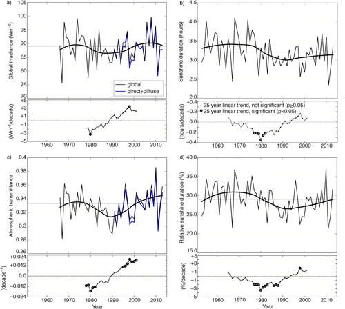
Fig. 5 As in Fig. 4. Time series of the a) cloud cover, b) cloud base, c) frequency of few or no clouds (NN<2 oktas), and d) frequency of low clouds with a cloud base height lower than 1000 m at the Florida (black lines) and Flesland (light blue lines) stations in Bergen, Norway.

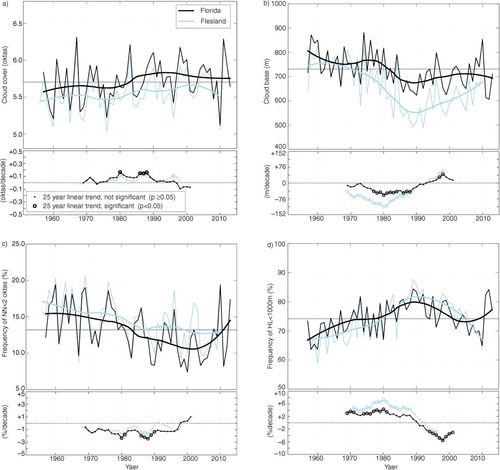
Fig. 6 Climatology of the (a) sunshine duration and (b) global irradiance measured at the Florida station in Bergen, and the (c) cloud cover, and (d) cloud base height, observed at both Florida and a second station, Flesland. In the upper panels, monthly climatologies are shown for the three 10-yr long periods 1965–1974 (circles), 1985–1994 (stars) and 2004–2013 (triangles).

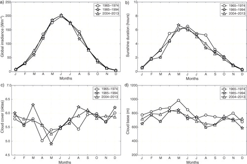
Fig. 7 Climatological change from (a, b, c, d) 1965–1974 to 1985–1994 and (e, f, g, h) 1985–1994 to 2004–2013 of the (a, e) global irradiance, (b, f) sunshine duration, (c, g) cloud cover, and (d, h) cloud base height. The monthly climatologies are shown in Fig. 6. The climatological change is estimated as the difference between the mean value for each month calculated for two periods. The statistical significance of the difference in mean value is evaluated by two-tailed t-test. Large markers represent differences between monthly mean values that are significant at the 95%-level (p<0.05).

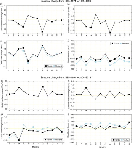
Fig. 8 Time series of (a) the aerosol optical depth, and (b) the diffuse fraction (diffuse/global irradiance). The AOD is calculated based only on hours when the sun is unobscured by clouds (sunshine duration=60 minutes), from diffuse and global irradiance (grey markers and lines) for the period 1965–2013, and from direct normal irradiance observations (blue markers and lines) for 1991–2013. The diffuse fraction is calculated based on diffuse and global irradiance for all hours, cloudy and clear. Small markers (in panel a) represent the monthly averaged AOD values, the solid lines (both panels) show the annual mean time series of AOD and diffuse fraction which is calculated based on the monthly values, and the dashed lines (in both panels) are local regression smoothed curves with a smoothing window of 30 yr. An increase in aerosol optical depth can be observed following the volcanic eruptions of El Chichón and Mount Pinatubo, which are marked in panel a.

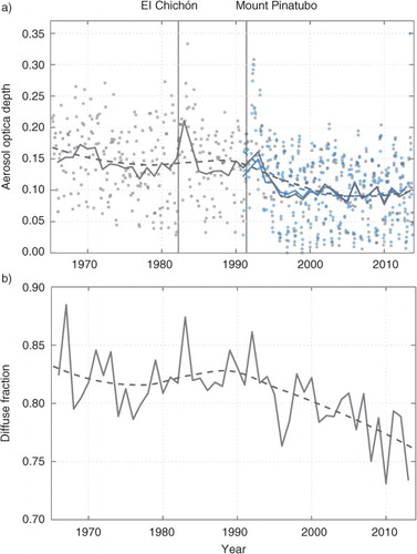
Fig. 9 Time series of (a) the observed surface air temperature in Bergen (combined measurements from the Florida and Fredriksberg sites) and (b) the average sea surface temperature anomaly of the North Atlantic Ocean.

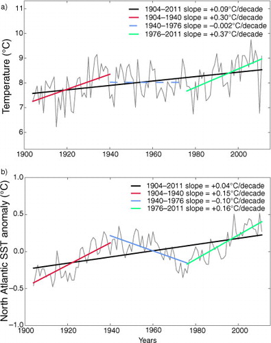
Table 1. Correlation (R) between the observed temperature (T), cloud cover (NN) and global irradiance (SW) in Bergen, calculated based on monthly mean time series for January–December as well as the annual and seasonal mean time series

Month	R(T, NN)	p	R(T, SW)	p	R(SW, NN)	p
January	+0.86	<0.0001	−0.82	0.0003	−0.83	0.0001
February	+0.77	0.0002	−0.75	0.001	−0.88	<0.0001
March	+0.41	0.07	−0.51	0.04	−0.94	<0.0001
April	+0.09	0.70	+0.04	0.88	−0.85	0.0002
May	−0.45	0.05	+0.36	0.15	−0.92	<0.0001
June	−0.63	0.003	+0.59	0.01	−0.94	<0.0001
July	−0.58	0.01	+0.52	0.05	−0.94	<0.0001
August	−0.54	0.02	+0.58	0.02	−0.96	<0.0001
September	−0.13	0.57	+0.08	0.75	−0.96	<0.0001
October	+0.40	0.10	−0.53	0.04	−0.85	<0.0001
November	+0.69	0.003	−0.56	0.02	−0.75	0.001
December	+0.81	<0.0001	−0.84	0.00001	−0.87	<0.0001
Annual mean	+0.35	0.14	+0.15	0.54	−0.72	0.003
Mar, Apr	+0.27	0.24	−0.18	0.47	−0.92	<0.0001
May–Aug	−0.53	0.02	+0.52	0.04	−0.91	<0.0001
Sep, Oct	−0.04	0.85	+0.14	0.58	−0.79	0.0007
Nov–Feb	+0.87	<0.0001	−0.71	0.004	−0.78	0.001

The correlation is estimated by the Pearson's correlation coefficient which has a range from −1 (perfect anti-correlation), via 0 (no correlation) to +1 (perfect correlation). The statistical significance of the correlation is estimated with a student's t-test and reported here as p, the probability of obtaining a given value of R from two independent time series. Correlation values that are statistically significant on the 95%-level (i.e p<0.05) are marked in bold font.

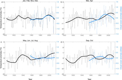
Fig. 10 Time series of observed air temperature in Bergen (black lines) and the average North Atlantic SST (blue lines). Thin lines represent the seasonal mean time series and thicker lines are smoothed Lowess curves. The panels show the seasonally averaged time series for (a) January, February, November and December, (b) March and April, (c) May, June, July and August, and (d) September and October. The seasons are defined based on the correlation between the temperature and cloud cover (Table 1), which is positive for November–February, negative for May–August, and for March, April, September and October, low and not statistically significant.

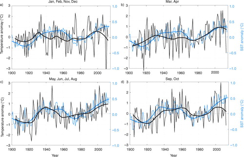
Fig. 11 Time series of temperature (black lines) and cloud cover (blue lines) measured at the Florida site in Bergen. Thin lines represent the seasonal mean time series and thicker lines are smoothed Lowess curves. The panels show the seasonally averaged time series for (a) January, February, November and December, (b) March and April, (c) May, June, July and August, and (d) September and October. The seasons are defined based on the correlation between the temperature and cloud cover (Table 1), which is positive for November–February, negative for May–August, and for March, April, September and October, low and not statistically significant.