On the use of MOZAIC-IAGOS data to assess the ability of the MACC reanalysis to reproduce the distribution of ozone and CO in the UTLS over Europe

Figures & data

Fig. 1 Map of MOZAIC flights for the studied period (2003–2010). The black square corresponds to the European region (40°N–55°N, 10°W–15°E) used in our study.

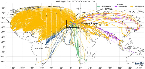
Fig. 2 Number of flights per month over the European region (Paris, London, Frankfurt, Munich, Düsseldorf and Vienna) from Jan 2003 to Dec 2010.

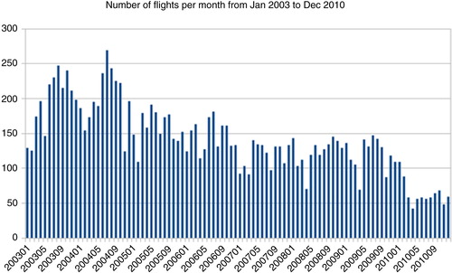
Fig. 3 Evolution of assimilated data and emissions sources (in blue cells) used in REAN from 2003 to 2010. MOPITT was used as anchor for CO and SBUV/2 data were used as anchor for ozone. Using SBUV/2 as anchor could not stop the bias correction drifting for individual MLS layers. When this was discovered during the reanalysis production, the bias correction was turned off for MLS and MLS was used uncorrected in REAN from 1 January 2008 onwards.

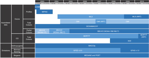
Fig. 4 Time series of monthly mean ozone (top) and CO (bottom) in the LS from January 2003 to December 2010, for REAN (red), CNTRL (green) and MOZAIC-IAGOS observations (blue). Standard deviations (2s) are given for REAN (orange contour), CNTRL (dark green contour) and MOZAIC-IAGOS observations (blue bars).

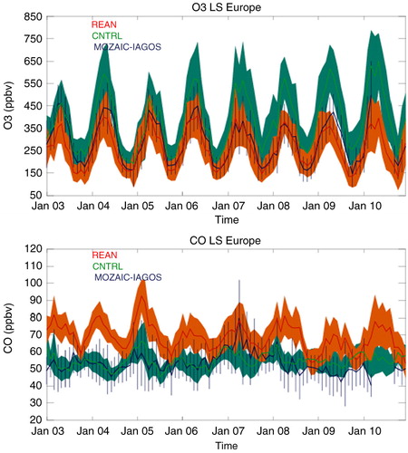
Fig. 5 Same as Fig. 2 for the UT.

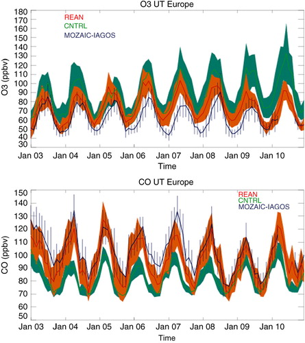
Fig. 6 Time series of LS minus UT differences of ozone (top) and CO (bottom) monthly means.

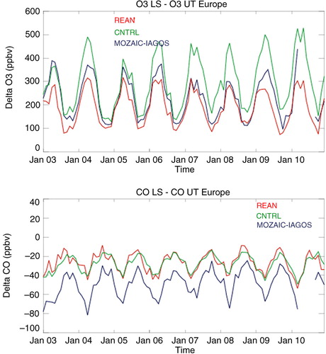
Fig. 7 Normalised Taylor diagrams for ozone (left) and CO (right) in the LS (top) and the UT (bottom) for both models REAN (red) and CNTRL (green), from 2003 to 2009. Years are referred in black (‘YY’) above each point. Point in blue (Obs) is the observation MOZAIC taken as the reference (R=1 and s=1). A perfect model would coincide with the observations at R=1, s=1. The minimum value for correlation in the figures is limited to zero, explaining missing data points in some cases.

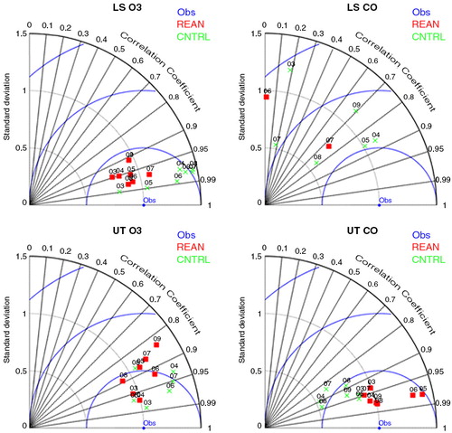
Fig. 8 Time series of annual means (solid) and associated trends (dashed) as linear fit calculated from annual mean anomalies of ozone and CO in the LS (top) and the UT (bottom) for REAN (red), CNTRL (green) and MOZAIC/IAGOS observations (blue) from January 2003 to December 2009. Overall linear trends are also indicated on the figure for the three datasets. The 2-sigma values are given to assess the uncertainty of the trends. The black line corresponds to an anomaly equal to zero.

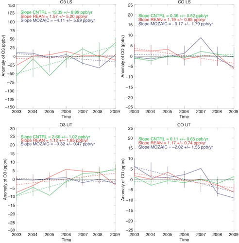
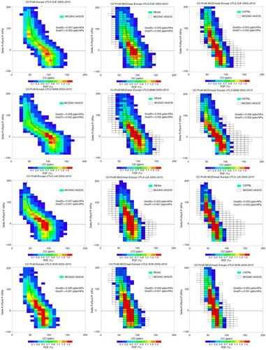
Fig. 9 Seasonal PDF of ozone as a function of CO in the Ex-UTLS for MOZAIC-IAGOS data averaged in a grid with horizontal resolution of 1.125° × 1.125° (first column), REAN (second column) and CNTRL (third column). The shape of the PDF for MOZAIC-IAGOS is reproduced on the model panels in black and white. The black lines correspond to the limits of the ‘low CO’ region, the ‘low O₃’ region and the extra tropical transition layer (ExTL) using seasonal thresholds of ozone (mean value of ozone in UT) and CO (mean value of CO in LS) in ppbv (blue on the panels).

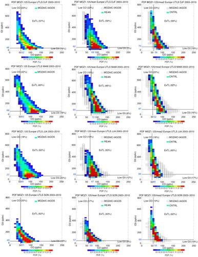
Fig. 10 Seasonal PDF of O₃ profile around the tropopause for the entire period 2003–2010 with pressure coordinate relative to the pressure level of the dynamical tropopause. As in Fig. 9, the first column is MOZAIC-IAGOS averaged in a grid with horizontal resolution of 1.125°×1.125°, the second column is REAN and the third column is CNTRL. The shape of the PDF for MOZAIC-IAGOS is reproduced on the model panels in black and white. Black lines correspond to mean profiles. GradS and GradT are the delta O₃ between 0 and 80 hPa above and below the dynamical tropopause.

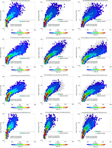
Fig. 11 Same as Fig. 10 for CO.