The IAGOS-CORE aerosol package: instrument design, operation and performance for continuous measurement aboard in-service aircraft

Figures & data

Fig. 1 Schematic setup of the IAGOS Aerosol Instrument. Aerosol particles are sampled using a quasi-isokinetic shrouded inlet by means of central vacuum unit (VAC). Flow rates through the individual instruments are kept constant by means of critical orifices. The double-walled container for butanol supply (BSC) and butanol reservoir (BRC) are statically pressurised to the inlet pressure. The exhaust of the VAC is connected to the sample outlet. In case of fire an overpressure of butanol is discharged via release valves connected to the outlet.

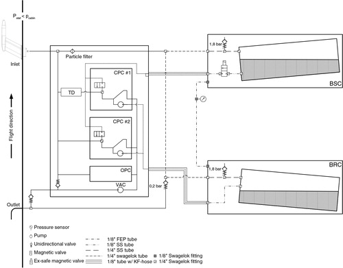
Table 1. Instrument components integrated in the IAGOS aerosol package

Instrument type	Instrument model		Size range	Time res.	Precision
Condensation particle counter	5.411 Sky Cpc	Cpc # 1	µm	1 s	±10 cm ^−3
Condensation particle counter
+ Thermodenuder at T=250° C	5.411 Sky Cpc	Cpc # 2	µm	1 s	±10 cm ^−3
Optical particle counter	1.129 Sky Opc	Opc	µm	1 s	±5 cm ^−3

Fig. 2 Schematic Sky OPC: The optical design is based on the wide-angle collection of light scattered under a mean scattering angle of 90 ° by means of a parabolic mirror which covers an angular range of 120 °. In addition, light scattered into an angular range of 18 ° is detected directly by the photodetector.

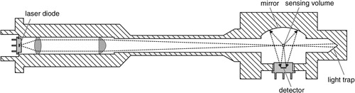
Fig. 3 Theoretical response function (depending on the given geometry of the OPC optics) calculated for different particle types [polystyrene latex (PSL), ammonium sulphate (AS) and di-ethyl-hexyl-sebacate (DEHS)].

Table 2. Lower limit for PSL, ammonium sulphate (AS) and di-ethyl-hexyl-sebacate (DEHS) per channel

Channel	PSL (µm)	AS (µm)	DEHS (µm)
1	0.250	0.263	0.284
2	0.280	0.294	0.320
3	0.300	0.318	0.348
4	0.350	0.370	0.412
5	0.400	0.426	0.474
6	0.450	0.488	0.566
7	0.500	0.555	0.658
8	0.580	0.626	0.717
9	0.650	0.710	0.891
10	0.700	0.800	0.934
11	0.800	0.862	1.050
12	1.000	1.089	1.254
13	1.300	1.300	1.450
14	1.600	1.600	1.640
15	2.000	2.000	2.000
16	2.500	2.500	2.500

Fig. 4 Schematic of a conductive cooling type Sky CPC. A sample flow is exposed to a butanol saturated environment called the saturator. Downstream of the saturator the flow is cooled in the condenser. Due to thermodynamical reasons a supersaturated butanol atmosphere is established. Here particles will grow by condensation. Thus, particles passing a laser beam are detected by their scattered light by means of a photo diode.

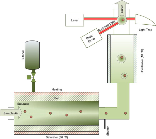
Fig. 5 The figure shows a comparison of extinction at a wavelength of 630 nm measured by the CAPS PM_ex instrument (y-axis) versus the extinction calculated for PSL spheres using the full size distribution information measured by the GRIMM OPC 1.129. During the experiment PSL nominal sizes and number concentration where varied. The regression line parameters for slope m and offset a as well as their standard deviation are shown.

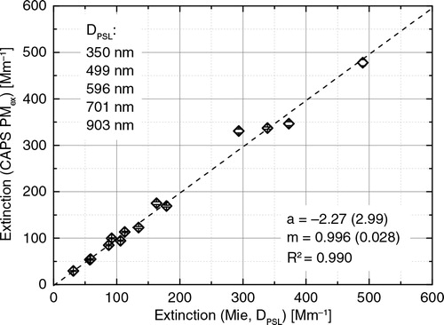
Fig. 6 OPC calibration using {299; 404; 499; 709 nm} PSL particles. The count probability which is defined by the channel count number divided by the total number of particles counted is plotted per OPC channel for two OPC instruments and for different PSL particles sizes. The response of an ideal OPC is added as hatched area.

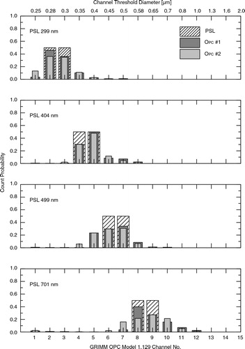
Fig. 7 This graph shows the instrument factor m for the IAGOS OPC (1.129) and for the non-modified predecessor OPC (1.109) as a function of the pressure. The factor m represents the instrumental calibration factor. Thus, size bin thresholds are defined by the product of m and the theoretical response function. The old design shows a significant pressure dependence whereas the modified IAGOS OPC (1.129) shows no significant pressure dependence of factor m.

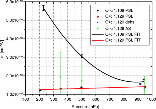
Fig. 8 OPC precision test: The plot shows the scatterplot of the total number concentration of two GRIMM Model 1.129 Sky-OPC instruments measuring laboratory test aerosols in a wide range of particle number concentration. In the plot the one-to-one correlation, the ±5 % margin and the linear regression parameters are shown.

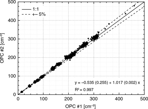
Fig. 9 This figure compiles ratios of number counts for individual sizing channels of two parallel measuring OPC. Considering the standard deviation indicated as error bars, the individual channels deviates from the one-to-one correlation significantly.

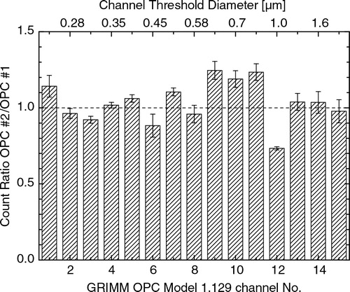
Table 3. Average ratio of number concentrations measured by two GRIMM Model 1.129 Sky-OPC instruments under different conditions; airborne measurements were performed during research flights in July 2008 over Greenland

Date	Aerosol type		Count ratio
28.08.2008	Laboratory air	Mean	1.003
		Sdev	0.014
29.08.2008	Ambient ground	Mean	1.014
		Sdev	0.012
04.09.2008	NaCl	Mean	1.023
		Sdev	0.008
04.09.2008	NaCl	Mean	1.026
		Sdev	0.026
02.07.2008	Ambient airborne	Mean	0.960
		Sdev	0.422

Fig. 10 The graph shows the calculated and measured temperature profiles along the thermodenuder centerline. The model-calculation is shown as a solid line and measurements are marked with an asterisk. Model calculation and measurements show similar results. The measurement deviates from calculation starting at 0.06 m distance which may be caused by microturbulence induced by the micro temperature sensor.

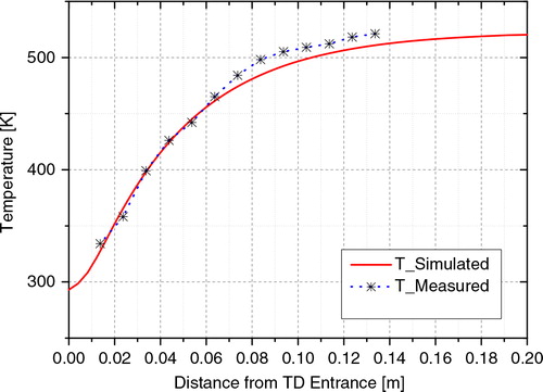
Fig. 11 Setup of the low pressure cut-off experiment. Particles are produced by means of a constant output atomizer Type TSI 3076. Particles are subsequently dried, charged and size selected by means of a DMA/americium diffusion charger. Monodisperse particles enter the low pressure section via a critical orifice and are further diluted by a particle free flow. The pressure in this section is actively controlled by means of a mass flow controller (MFC). An aerosol splitter provides the aerosol flow for the test candidate CPC and the reference instrument FCE.

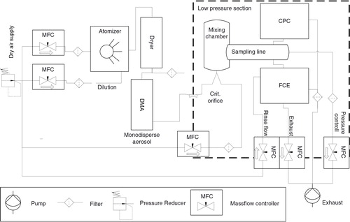
Fig. 12 This graph shows the measured volume flux QA limited by the critical orifice as a function of the pressure of the sampling line (with respect to ambient pressure of 1013 hPa) during the experiment.

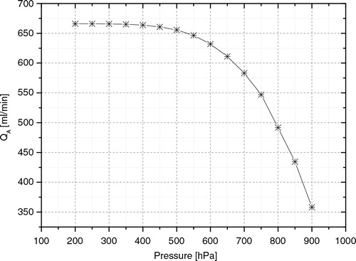
Table 4. Approximation coefficients a _i (n)

	n
a i (n)	−2	−1	0	1	2
a 0	−26.3328	−2.3197	−0.0003	−2.3484	−44.4756
a 1	35.9044	0.6175	−0.1014	−0.6044	79.3772
a 2	−21.4608	0.6201	0.3073	0.4800	−62.8900
a 3	7.0867	−0.1105	−0.3372	0.0013	26.4492
a 4	−1.3088	−0.1260	0.1023	−0.1544	−5.7480
a 5	0.1051	0.0297	−0.0105	0.0320	0.5059

Fig. 13 The graph shows the multi-charge correction factor ξ(D_p) as a function of the particle diameter. The red line shows the first order approximation ignoring the actual size distribution by setting C =1. The first order approximation deviated significantly (up to 15 %) from the ξ(D_p) curve. Thus, the actual size distribution measurement has to be considered calculating parameter C .

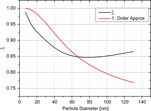
Fig. 14 CPC accuracy test: The graph shows the scatterplot of number concentrations measured with the GRIMM CPC versus the reference GRIMM FCE. The one-to-one correlation as well as ±5 % boundaries and the linear regression analysis is shown.

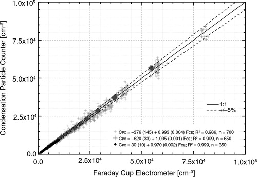
Fig. 15 CPC precision test: The scatterplot of two identical CPC instruments of type GRIMM 5.411 are shown. The number-density of NaCl particles are varied in the range up to 20 000 particle per cm⁻³.

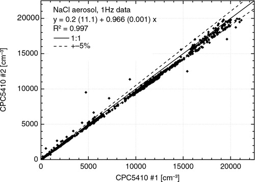
Fig. 16 This graph shows the CPC counting efficiency ξ(D_p) as a function of the particle diameter compiling results for 170, 200, 600 and 900 hPa pressure levels.

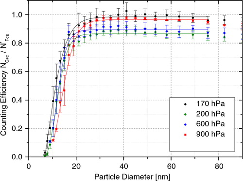
Table 5. Cut-off diameter as function of ξ for the given pressure level

Pressure (hPa)	a	Δa	b	Δb	D 1 (nm)	ΔD 1 (nm)	D 2 (nm)	ΔD 2 (nm)	x ^2	r ^2	D 50 (nm)	D 50s (nm)
170	0.985	0.006	1.662	0.256	8.180	1.131	3.666	0.345	4.95E-04	0.995	11.4	1.1
200	0.866	0.006	0.985	0.044	11.860	0.282	2.322	0.188	4.68E-04	0.995	13.1	0.9
600	0.895	0.007	1.079	0.288	11.547	1.267	2.230	0.433	7.62E-04	0.979	12.8	0.9
900	0.966	0.006	1.106	0.097	13.942	0.607	2.942	0.288	4.52E-04	0.994	14.9	1.1