Figures & data
Fig. 1 Location and photograph of fixed platform.
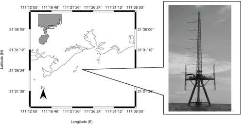
Fig. 2 Example spectra of velocity fluctuations for 8-min record, where S v corresponds to that of vertical velocity, partitioned into wave motion and turbulence parts. S h corresponds to that of the horizontal velocity, which was multiplied by a factor of 100 for clarity. A fit to S v in the inertial subrange is overlaid.
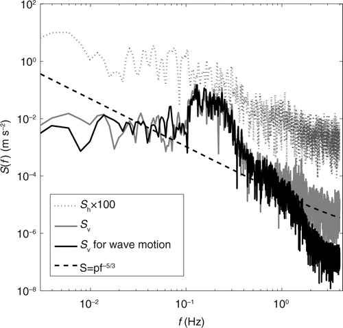
Fig. 3 Example of wave frequency spectrum derived from AWAC data.
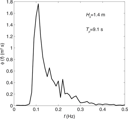
Fig. 4 Vertical distribution of ɛ: (a) ɛH
s/u*w versus z/H
s and (b) versus z/H
s.
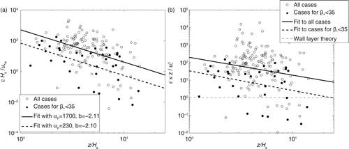
Fig. 5 Locations of buoys from National Buoy Data Center.
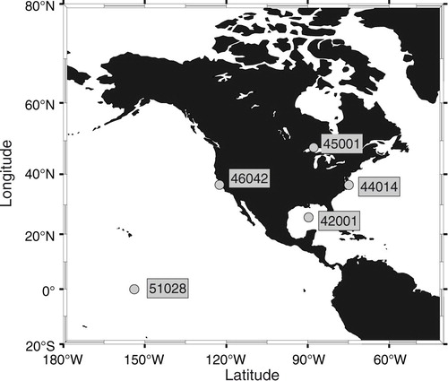
Fig. 6 The plot of non-dimensional wave height versus non-dimensional wave period.
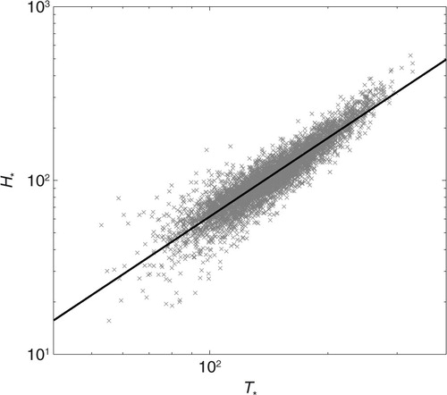
Table 1. Buoys’ information
Fig. 7 Breaking wave-energy dissipation rates as functions of U 10 (a) and R B (b). The small circles in the figure denote the data from Felizardo and Melville (Citation1995).
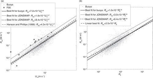
Fig. 8 Probability distribution of wave age.
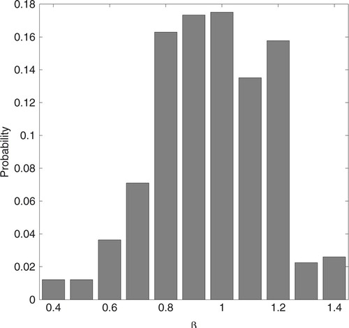
Fig. 9 Field (GaxEx-1998) and laboratory comparisons of k L for (a) CM, (b) Z03, (c) W05 and (d) M01.
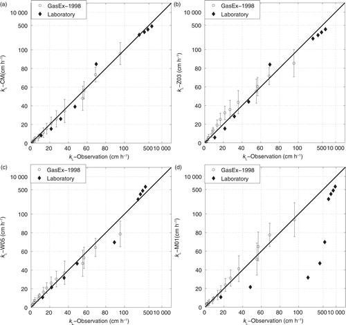
Table 2. Analytic statistics for gas transfer velocities estimated from different models: CM (composite model), Z03 (Zhao et al., 2003), W05 (Woolf, Citation2005) and M01 (McGillis et al., Citation2001)
Fig. 10 Gas transfer velocity as function of wind speed from CM and other U 10-based models.
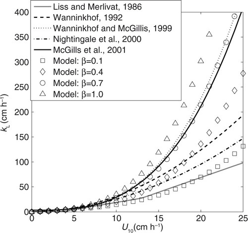
Fig. 11 Gas transfer velocity for ‘breaking’ and ‘non-breaking’ as a function of wind speed.
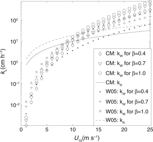
Fig. 12 The domain (square) of the numerical simulation.
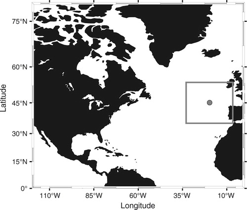
Fig. 13 Comparison of U 10 values between GasEx-1998 and CCMP.
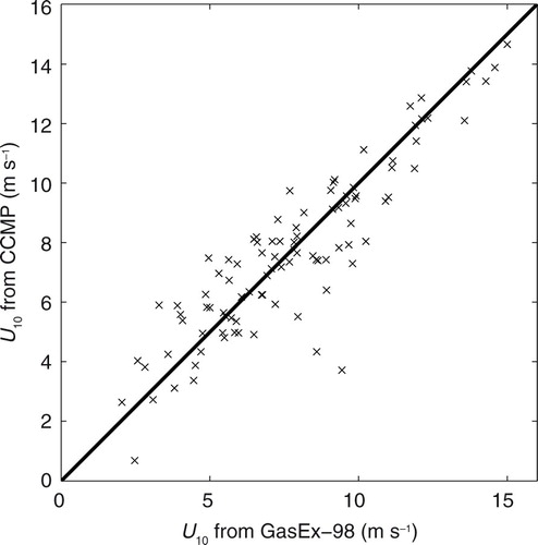
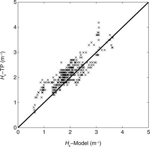
Fig. 14 Comparison of H s values between along-track altimeter and wave model.