The first twenty years (1994–2014) of ozone soundings from Rapa Nui (27°S, 109°W, 51 m a.s.l.)

Figures & data

Fig. 1 Location (left) and main topographic features (right) of Rapa Nui or Easter Island. The right panel also shows the main roads (white) and the town of Hanga Roa in Rapa Nui (red).

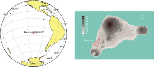
Fig. 2 Seasonal and annual ozone sounding sampling at Rapa Nui between 1994 and 2014. The dashed black line shows the number of soundings launched per year. The continuous line indicates the number of valid soundings reaching up to 15 km altitude. The bars show the corresponding distribution per season.

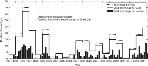
Table 1. Number of ozone soundings analysed in this study per year and season

Year	DJF	MAM	JJA	SON	Total
1994	0	0	0	3	3
1995	7	2	6	7	22
1996	6	11	10	7	34
1997	6	10	4	0	20
1998	2	0	0	3	5
1999	1	4	9	4	18
2000	1	0	0	0	1
2001	3	2	0	0	5
2002	0	0	0	0	0
2003	0	0	0	3	3
2004	0	7	5	2	14
2005	0	2	6	5	13
2006	1	3	2	0	6
2007	1	3	6	0	10
2008	1	3	1	0	5
2009	1	3	7	3	14
2010	1	3	7	1	12
2011	0	0	0	0	0
2012	1	0	3	4	8
2013	1	3	10	4	18
2014	2	5	12	4	23
Total	35	61	88	50	234

Seasons correspond to: summer (December–January–February, DJF); fall (March–April–May, MAM); winter (June–July–August, JJA); and spring (September–October–November, SON).

Fig. 3 Precipitation, boundary layer winds (at 925 hPa) and surface pressure affecting Rapa Nui. Rapa Nui (27°S, 109°W) is indicated by a black dot. Wind vectors are shown as arrows, including for reference the 12 m/s wind speed. The shaded field corresponds to precipitation in mm/season. The subtropical high is indicated by surface isobars larger than 1018 hPa. Data source: NCEP/NCAR reanalysis.

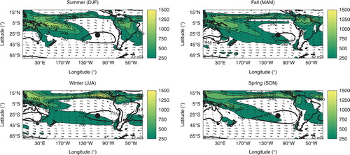
Fig. 4 Subtropical jet stream, surface temperature and subsidence in the Pacific along the year. Arrows show wind velocity in excess of 25 m/s at 200 hPa. Surface temperatures in °C (at 1000 hPa) are also shown. The area with omega velocities in excess of 4 hPa/s, that is, regions of prevailing subsidence are indicated with a black line. The black dot indicates the location of Rapa Nui. Data: NCEP/NCAR Reanalysis.

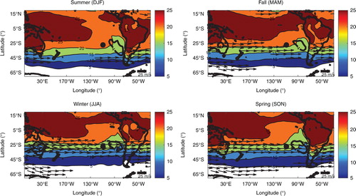
Fig. 5 Seasonal cycles of vertical velocity (in hPa/s, left panel), zonal wind (in m/s, middle panel) and potential vorticity (in PVU=10⁻⁶ m⁻²s⁻¹K kg⁻¹, right panel) over Rapa Nui. Data: NCEP/NCAR Reanalysis.

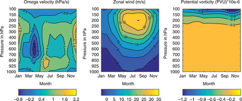
Fig. 6 Precipitation (in mm/month, left panel), surface temperature (in °C, middle panel) and outgoing long-wave radiation (OLR, in W/m², right panel) climatologies over Rapa Nui for the period 1994–2014. Precipitation and temperature were obtained from the Chilean Weather Office. OLR values obtained from NCEP/NCAR reanalysis. Data are presented as box plots: the central mark in the box indicates the median of the distribution, the edges of the box are the 25th and 75th percentiles, the whiskers extend to the most extreme data points not considered outliers, and outliers are plotted individually (red crosses).

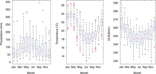
Fig. 7 Seasonal cycles of ozone in ppbv (left) and specific humidity in g/kg (right) vertical profiles for the period 1994–2014. Isolines and colour codes are shown in the figure. The chemical tropopause, that is, 100 ppbv is indicated in the left panel by a coarse black line. For accuracy, specific humidity, which is derived from relative humidity measurements, is drawn only below 6 km.

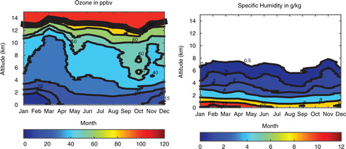
Fig. 8 The upper left panel shows the seasonal variation in tropospheric ozone column (TOC) in Dobson Units (DU=2.69×10¹⁶ ozone molecules per square cm). The upper right panel illustrates the thermal tropopause height (TT) in km. The lines indicate the corresponding climatologies derived from the OMI/MLS and the TOMS/SBUV satellite products (dashed lines) in black and red, respectively. The lower left panel shows the seasonal variation of carbon monoxide (CO) in ppbv and the lower right panel illustrates the seasonal variation of beryllium 7 radionuclide (⁷Bel) in mBq/m³ measured at Rapa Nui. These are the box plots of monthly averages using the same convention as in Fig. 6. Data sources: NOAA/ESRL/GMD (CO for the period 1994–2013); EML (7Be for the period 1971–1999); CCHEN (⁷Be for the period 2009–2014).

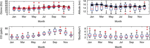
Fig. 9 Tropospheric ozone column (TOC) as derived from individual soundings (red dots), and monthly averaged satellite products: TOMS/SBUV (blue dashed line) and OMI/MLS (blue continues line). The grey-dashed areas correspond to spring periods. TOMS/SBUV data were obtained from www.science.larc.nasa.gov/TOR/data.html. OMI/MLS data were downloaded from www.acd-ext.gsfc.nasa.gov/Data_services/cloud_slice/.

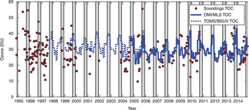
Fig. 10 Ozone profiles (upper left panel), seasonality (lower left panel) and vertical (upper right panel) and horizontal (lower right panel) trajectories for group 1 (G1) according to SOM classification of Rapa Nui ozone soundings. The average of all soundings (trajectories) is indicated by the continuous blue line, and the cluster average is shown by the dashed red line. Individual profiles (trajectories) are shown in grey. Trajectories were calculated using HYSPLIT fed with NCEP/NCAR reanalysis data.

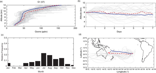
Fig. 11 As in Fig. 10 but for group 2 (G2).

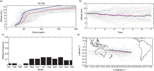
Fig. 12 As in Fig. 10 but for group 3 (G3).

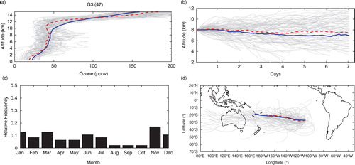
Fig. 13 As in Fig. 10 but for group 4 (G4).

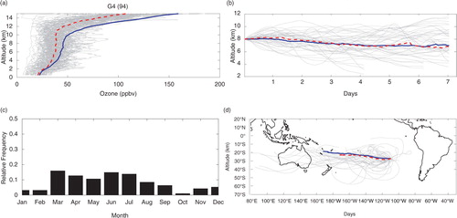
Fig. 14 Classification of ozone profiles according to self-organising maps of back trajectories. From left to right, resulting groups, GA and GB, and number of members in parenthesis. From top to bottom, the two upper panels show the horizontal and vertical projections of individual back trajectories (light grey lines), average back trajectory for all soundings (solid blue) and group representative (dashed red line). The two lower panels show the relative frequency of occurrence of the back trajectories, and the corresponding individual ozone profiles (light grey lines), average of all ozone soundings (blue line) and average ozone profile for the group (dashed red line).

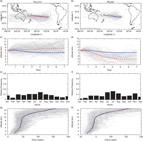
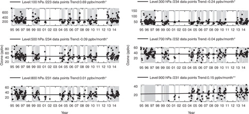
Fig. 15 Trend analysis for ozone at Rapa Nui. Linear trends shown by a continuous black line are calculated for isobaric levels indicated in each panel. The number of data points and the corresponding trend are also indicated. Grey lines show individual soundings.