Coupling an aerosol box model with one-dimensional flow: a tool for understanding observations of new particle formation events

Figures & data

Fig. 1 A banana-shaped new particle formation event observed at the Sammaltunturi measurement site in the Pallas-Sodankylä GAW station 5–6th of September 2000. The x-axis is time in day-of-year and particle number concentration in each size class is given with colour in dN/dlog₁₀ D _p.

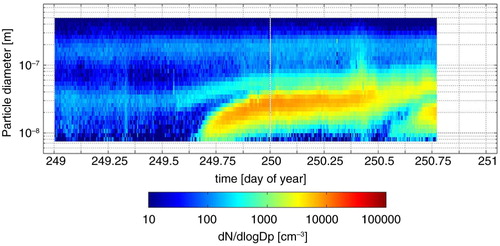
Fig. 2 Schematic of the LMASON model. The t _i values represent the time at time step i. Note the wind speed change between t₃ and t₄ affecting the distance that the boxes move between time steps. The particle size distribution in each box as it advects over the measurement site provides the simulated observations (on the right).

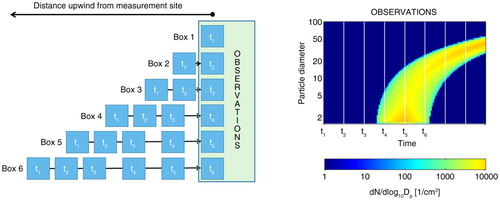
Fig. 3 Plot of a new particle formation event provided by the LMASON model output. This event is only limited temporally [T_J1.5(t)>0 between hours 8 and 16, all other parameters are constant]. Panels on the left show the input values for S_J1.5(X) and S_GR(X) (top), T_J1.5(t) and T_GR(X) (middle) and WS (bottom). On the right, the top panel shows the evolution of the particle number size distribution (PNSD) as a function of time over 2 days, with particle number concentrations in each bin given as colour in dN/dlog₁₀ D _p. The second panel shows the number concentration of particles with D _p<150 nm as a function of time. The third panel shows the formation rate, J _1.5, as calculated from the output PNSD data and compared to the input values. The lowest panel shows particle growth rates as a function of time calculated from the output PNSD data using mode peak diameter at each time point (vertical) and times of maximum particle number concentration in each size class (horizontal), and the input growth rate at the measurement site as a function of time.

Fig. 4 New particle formation limited spatially only [constant T_J1.5(t)] taking place 200–400 km upwind of the measurement site) starting at t=0. The figure panels are the same as in Fig. 3.

Fig. 5 Two very similar simulated observations from different input conditions. The figure explanations are as in Fig. 3. (a) shows new particle formation taking place between hours 12 and 20 more than 70 km upwind of the measurement site. Particle growth rate is constant and wind speed is constant 50 km h⁻¹. (b) shows new particle formation taking place between hours 8 and 16 more than 270 km upwind of the measurement site. Particle growth in the closest 270 km is lower than that beyond this limit. Wind speed is again constant 50 km h⁻¹.

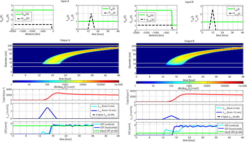
Fig. 6 The change of peak particle diameter ΔD_p of the growing mode between times t and t+Δt extracted from an observed new particle formation event, and the corresponding change in location where the observed particles were formed ΔX along a trajectory upwind of the measurement site (marked with a star). The new particle formation event in the figure is the same one as in Fig. 1.

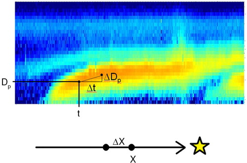
Fig. 7 A new particle formation event with temporal changes in particle growth rate at hours 16 and 32 [T _GR(t) changing, S _GR(X) constant]. The figure explanations are as in Fig. 3.

Fig. 8 A new particle formation event where growth rate changes as a function of location (from t=14 to t=20 hours) and as a function of time (at t=24 hours). Notice the observable growth continuing after 24 hours, even though GR(t,X)=0.

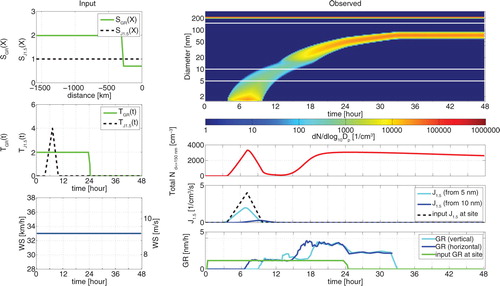
Fig. 9 How changes in wind speed affect observations of different new particle formation events. The figure explanations are as in Fig. 3. (a) shows a spatially and temporally limited new particle formation event with decreasing wind speed and (b) shows a spatially limited new particle formation event with decreasing wind speed, resulting in a ‘false banana’.

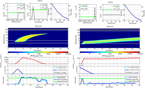
Fig. 10 An observed new particle formation event at the Sammaltunturi site in Pallas-Sodankylä GAW station 15–16th of July 2011. The black circles represent the evolution of particle diameter (1-hour sliding average of diameter of the size bin with highest particle concentration in dN/dlog₁₀ D _p). A period of mostly decreasing particle size can be seen between hours 17 and 30.

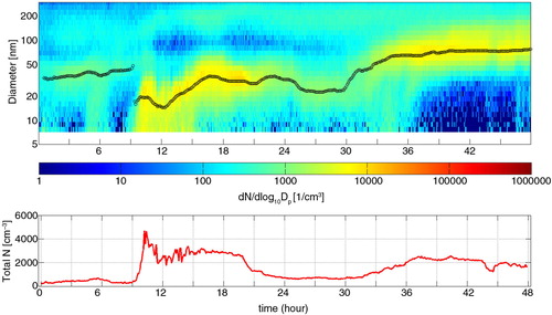
Fig. 11 Simulation of the observed event presented in Fig. 10 using both a temporally and spatially varying growth rate. Figure explanations are as in Fig. 3. The yellow line in the upper right panel is the evolution of the peak diameter in Fig. 10.

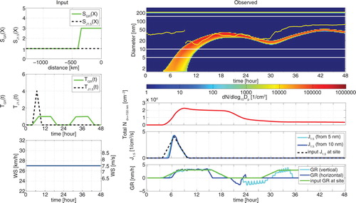
Table 1. Effects of doubling different input parameters on the observable parameters of the growing mode at the measurement site in a temporally limited (‘banana type’) NPF event

Changing parameter	Change in GR(t)obs of the mode	Change in N Dp<150 nm of the mode	Change in diameter width of the mode
2×S J1.5(X) upwind	No effect	2×	No clear effect
2×TGR(t)	2×	No clear effect	No clear effect
2×SGR(X) upwind	2×	Increase	2×

The effects are described as if they occur in the observable data after the formation of new particles has ceased. The direction of the spatial changes is towards upwind of the site.