Radon as a tracer of atmospheric influences on traffic-related air pollution in a small inland city

Figures & data

Fig. 1 Close-up of Bern town centre, showing the location of the radon (R), pollution (A), traffic (B) and meteorological (C) monitoring stations. Small inset shows the location of the measurements within the broader Bern city area. Black lines are railway lines (electric). Map data were obtained from OpenStreetMap (www.openstreetmap.org) and enhanced with Corine Land Cover information (Bosard et al., 2000).

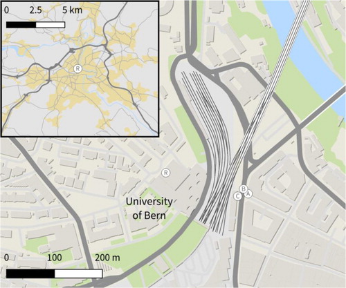
Fig. 2 (a) Diurnal composite of the diurnal-only component of the entire 13-month Bern radon time series; (b) cumulative frequency histogram of mean radon concentrations within the 12-hour ‘stability window’ each night, with quartile ranges indicated; and (c) diurnal composite near-surface radon concentrations corresponding to four atmospheric stability categories defined using the quartiles.

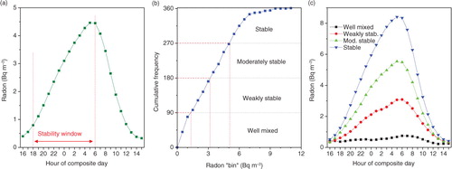
Fig. 3 (a) Diurnal composites of the diurnal-only component of Bern radon concentrations in summer and winter; and (b) seasonal radon accumulation curves at Bern referenced to the 1900 h radon concentration.

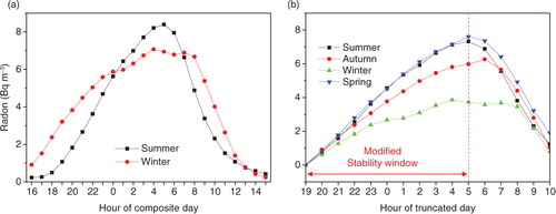
Fig. 4 Seasonal comparison (winter and summer) of Bern diurnal traffic density (passenger cars and trucks) for weekdays, Saturdays and Sundays.

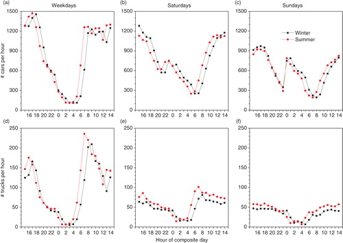
Fig. 5 Diurnal cycles of Bern total traffic density as a function of season (winter and summer), day of week and atmospheric stability.

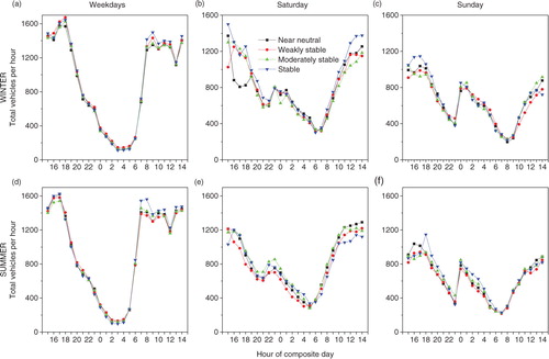
Fig. 6 (a, b, c, e, f) Monthly distributions (10/50/90th percentiles) of hourly meteorological and pollutant observations; and (d) monthly mean observed, fetch-related and diurnal components of Bern radon data.

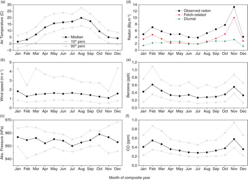
Fig. 7 Hourly mean diurnal composites by season: (a) diurnal radon, (b) total traffic density (cars + trucks), (c) benzene and (d) CO. Results are for weekdays only.

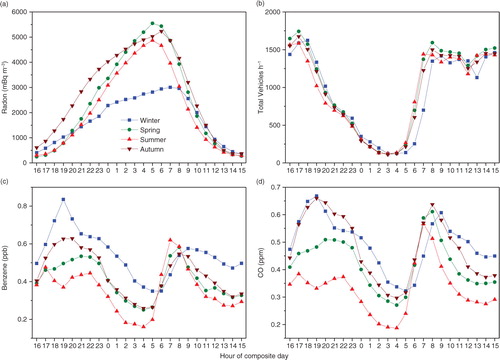
Fig. 8 Diurnal temperature (relative to the morning minimum value) at Bern in winter and spring as a function of radon-derived stability category.

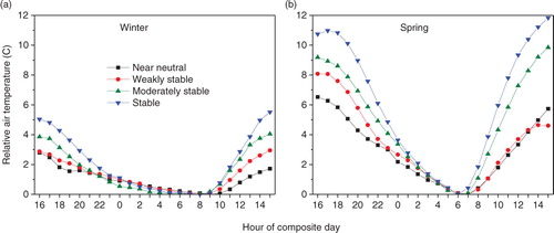
Fig. 9 Seasonal breakdown of the change in daily mean cloud cover with stability classification (1: well mixed/near neutral; 2: weakly stable; 3: moderately stable; 4: very stable).

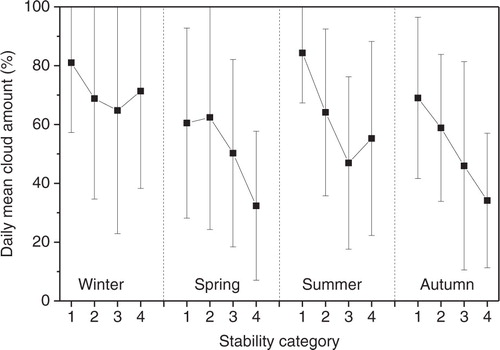
Fig. 10 Hourly mean diurnal composites of wind speed by season and stability classification.

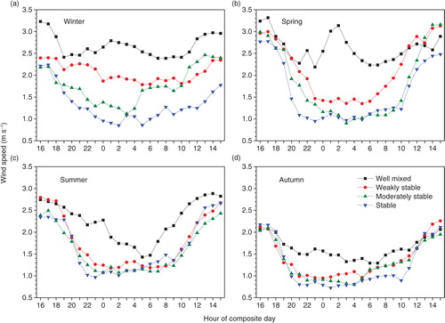
Fig. 11 Hourly mean diurnal composites of benzene concentration by season and stability category (weekdays only).

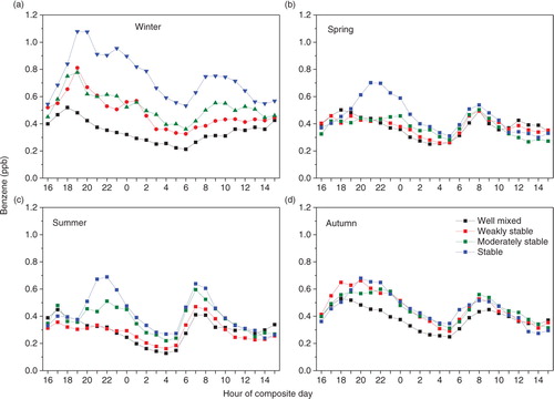
Fig. 12 Hourly mean diurnal composites of carbon monoxide concentration by season and stability category (weekdays only).

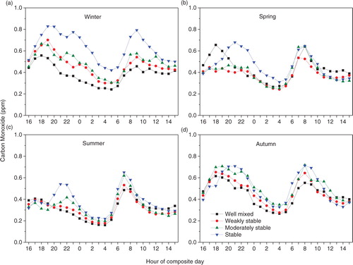
Fig. 13 Seasonally separated nocturnal composites of (a, b) radon concentrations, (c, d) box-model-derived SNBL depths (note logarithmic scale), (e, f) wind speed and (g, h) wind direction, for very stable (left) and weakly stable (right) conditions in Bern.

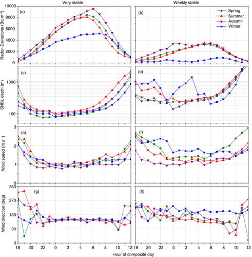
Fig. 14 Least-squares regression coefficients of the correlation between pollutant fluxes (CO; benzene) computed by the box model and measured total vehicle counts in Bern city centre, for a range of values of the spatial decay parameter γ _x (expressed as a half-distance). Only very stable nights in spring were used in these tests, and pollutant half-lives were held constant at 20 d for CO and 13 d for benzene. Optimised γ _x values used in the box model are indicated with vertical dashed lines.

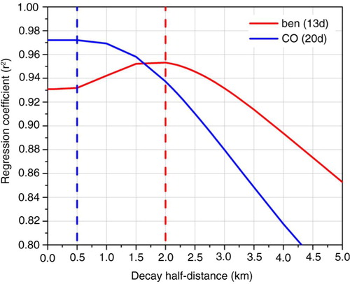
Fig. 15 Box model results for benzene in Spring ‘very stable’ conditions in Bern. (a) Time series of computed benzene flux on right axis and measured total vehicle counts (TVC) on left axis; also shown is computed SNBL depth, h, on left axis; (b) computed benzene flux versus measured TVC during the period 2000–0600 h, marked with vertical dashed lines in (a). Linear fit is indicated in red; inset shows the entire period 1800–1200 h.

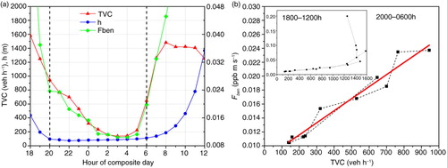
Fig. 16 Comparison of box model behaviour with (a, c) and without (b, d) horizontal advection, for Spring ‘very stable’ conditions. (a, b) Component terms for layer-integrated benzene (P _ben h) over the extended period 1800–1200 h, using pre-estimated fluxes (F _ben ) and radon-based SNBL depths (h). F _ben was calculated from TVC using regression results from the full model during the well-simulated period 2000–0600 h. (c, d) Modelled and measured P _ben and h values.

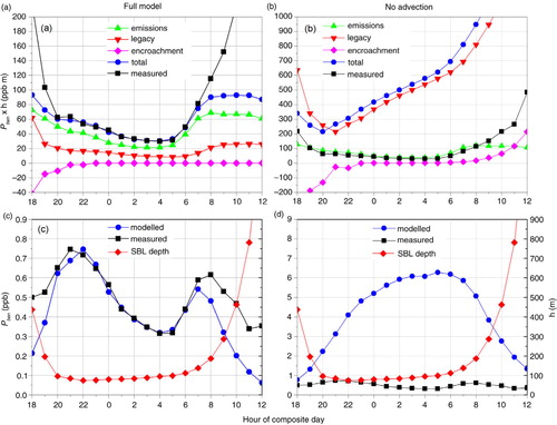
Table 1. Regression results for box-model-simulated pollutant fluxes (F _x ) versus measured total vehicle count (TVC) in Bern, by stability category and season

		Regression coefficient (r^2)				Gradient [F x ] per [veh h^−1]				Offset [F x ]
Regression (F x vs. TVC)	Stability category	Spring	Summer	Autumn	Winter	Spring	Summer	Autumn	Winter	Spring	Summer	Autumn	Winter
	Weakly stable	0.9300	0.8099	0.8124	0.3998	0.4954	1.2057	0.5546	3.7596	284.1	−10.6	205.2	773.4
Benzene flux	Moderately stable	0.9002	0.9382	0.8446	0.5163	0.3472	0.6825	0.2090	0.2639	78.1	66.4	233.6	587.1
F b [µg m^−2 h^−1]	Very stable	0.9532	0.9603	0.9699	0.8439	0.1987	0.5063	0.2948	0.3405	93.6	55.6	71.7	202.4
	Weakly stable	0.9019	0.8185	0.8185	0.3051	0.5750	1.4922	0.7314	3.6271	491.8	107.4	337.1	1464.7
CO flux	Moderately stable	0.8759	0.9686	0.8494	0.6007	0.4970	0.6246	0.2871	0.3244	131.6	158.7	377.6	746
F c [mg m^−2 h^−1]	Very stable	0.9720	0.9756	0.9388	0.9243	0.2241	0.4650	0.3796	0.3752	145.5	113.5	138.1	230.5

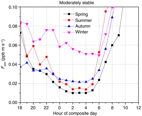
Fig. 17 Simulated benzene fluxes for Bern in moderately stable conditions by season.

Bosard M. , Feranec J. , Otahel J . CORINE land cover technical guide – addendum 2000. European Environmental Agency Technical Report. 2000. No. 40, Copenhagen, Denmark.

 Google Scholar