666
Views
6
CrossRef citations to date
0
Altmetric
Application Papers

Modeling the Potential Impacts of Climate Change on a Small Watershed in Labrador, Canada

Pages 231-251 | Published online: 23 Jan 2013

Figures & data

Figure 1. Churchill River basin and Pinus River sub-basin.

Figure 1. Churchill River basin and Pinus River sub-basin.

Table 1. Details of NARCCAP's RCMs and GCMs.

Table 2. NARCCAP ensemble members used.

Figure 2. Measured and WATFLOOD simulated daily average flows.

Figure 2. Measured and WATFLOOD simulated daily average flows.

Figure 3. Examples of base period simulated precipitation bias corrections for the CRCM-CGCM3 ensemble member (left) and a comparison of normalized precipitation bias for the range of models (right).
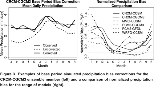
Figure 3. Examples of base period simulated precipitation bias corrections for the CRCM-CGCM3 ensemble member (left) and a comparison of normalized precipitation bias for the range of models (right).

Figure 4. Examples of base period simulated temperature bias corrections for the CRCM-CGCM3 ensemble member (left) and a comparison of normalized temperature bias for the range of models (right).
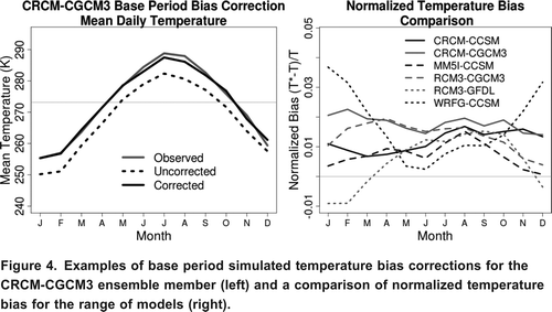
Figure 4. Examples of base period simulated temperature bias corrections for the CRCM-CGCM3 ensemble member (left) and a comparison of normalized temperature bias for the range of models (right).

Figure 5. Changes in daily precipitation from simulated base period to future period. Ensemble mean represented by thick black line.
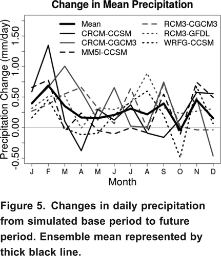
Figure 5. Changes in daily precipitation from simulated base period to future period. Ensemble mean represented by thick black line.

Table 3. Mean monthly and annual changes in precipitation rates.

Figure 6. Probability density functions for ensemble daily mean (top left), five-day mean (top right), monthly mean (bottom left) and annual precipitation rates (bottom right).
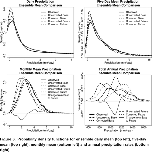
Figure 6. Probability density functions for ensemble daily mean (top left), five-day mean (top right), monthly mean (bottom left) and annual precipitation rates (bottom right).

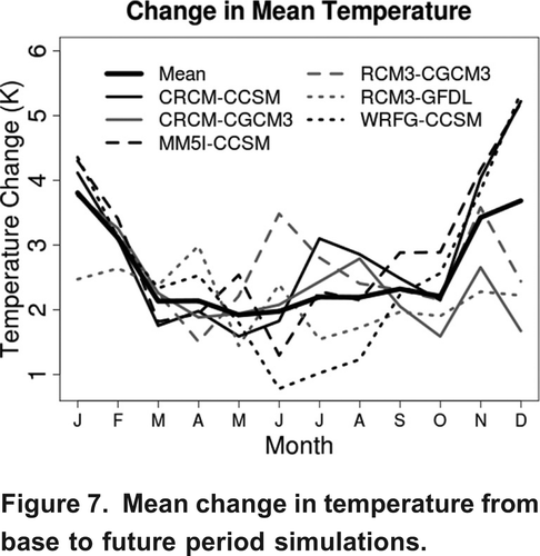
Figure 7. Mean change in temperature from base to future period simulations.

Figure 7. Mean change in temperature from base to future period simulations.

Table 4. Mean monthly and annual increases in temperature.

Figure 8. Probability density functions for ensemble daily mean (top left), five-day mean (top right), monthly mean (bottom left) and annual temperature (bottom right).
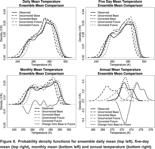
Figure 8. Probability density functions for ensemble daily mean (top left), five-day mean (top right), monthly mean (bottom left) and annual temperature (bottom right).

Figure 9. Examples of mean streamflow for the base (left) and future periods (right) from the corrected CRCM3-CGCM3 ensemble member. 30-year mean streamflow represented by black points.
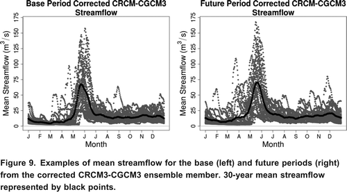
Figure 9. Examples of mean streamflow for the base (left) and future periods (right) from the corrected CRCM3-CGCM3 ensemble member. 30-year mean streamflow represented by black points.

Figure 10. Comparison of 30-year ensemble mean simulated base and future period streamflow (left) and the change in 30-year ensemble mean simulated streamflow (right), from base to future period.
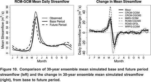
Figure 10. Comparison of 30-year ensemble mean simulated base and future period streamflow (left) and the change in 30-year ensemble mean simulated streamflow (right), from base to future period.

Table 5. Mean monthly and annual changes in streamflow.

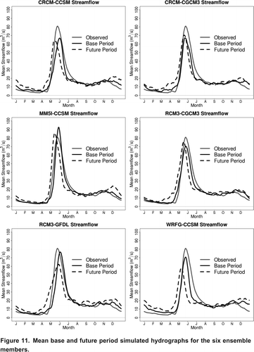
Figure 11. Mean base and future period simulated hydrographs for the six ensemble members.

Figure 11. Mean base and future period simulated hydrographs for the six ensemble members.

Figure 12. Probability density functions of mean annual flows for ensemble members during the base period (left) and the ensemble means (right) for base and future periods.
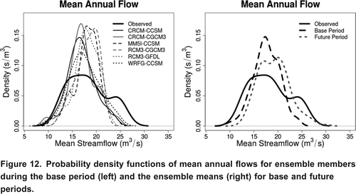
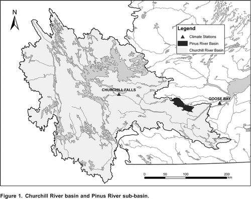
Figure 12. Probability density functions of mean annual flows for ensemble members during the base period (left) and the ensemble means (right) for base and future periods.
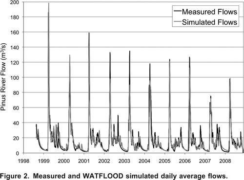
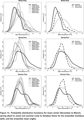
Figure 13. Probability distribution functions for mean winter (November to March), spring (April to June) and summer (July to October) flows for the ensemble members (left), and the ensemble mean (right).

Figure 13. Probability distribution functions for mean winter (November to March), spring (April to June) and summer (July to October) flows for the ensemble members (left), and the ensemble mean (right).

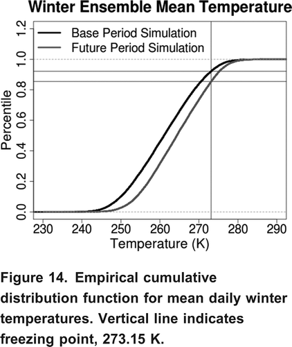
Figure 14. Empirical cumulative distribution function for mean daily winter temperatures. Vertical line indicates freezing point, 273.15 K.

Figure 14. Empirical cumulative distribution function for mean daily winter temperatures. Vertical line indicates freezing point, 273.15 K.

Reprints and Corporate Permissions

Please note: Selecting permissions does not provide access to the full text of the article, please see our help page How do I view content?

To request a reprint or corporate permissions for this article, please click on the relevant link below:

Academic Permissions

Please note: Selecting permissions does not provide access to the full text of the article, please see our help page How do I view content?

Obtain permissions instantly via Rightslink by clicking on the button below:

If you are unable to obtain permissions via Rightslink, please complete and submit this Permissions form. For more information, please visit our Permissions help page.