
Abstract
In this paper, we first give a brief survey on the power domination of the Cartesian product of graphs. Then we conjecture a Vizing-like inequality for the power domination problem, and prove that the inequality holds when at least one of the two graphs is a tree.
1 Introduction
Electrical power companies are required to continually monitor the state of their system as defined by a set of variables, for example, the voltage magnitude at loads and the machine phase angle at generators [Citation1]. These variables can be monitored by placing phase measurement units (PMUs) at selected locations in the system. Due to the high cost of a PMU, it is desirable to monitor (observe) the entire system using the least number of PMUs.
To model this optimization problem as a power domination problem, we use a graph to represent an electrical network. A vertex denotes a possible location where PMU can be placed, and an edge denotes a current carrying wire. A PMU measures the state variable (voltage and phase angle) for the vertex at which it is placed and its incident edges and their ends. All these vertices and edges are said to be observed by the PMU. We can apply Ohm’s law and Kirchoff’s current law to deduce the other three observation rules:
| 1. | Any vertex that is incident to an observed edge is observed. | ||||
| 2. | Any edge joining two observed vertices is observed. | ||||
| 3. | For | ||||
We consider only graphs without loops or multiple edges. Let be a graph with vertex set
and edge set
. A spanning subgraph of a graph
is a graph whose vertex set is the same as that of
, but its edge set is a subset of that of
. The neighborhood
of a vertex
is the set of all vertices adjacent to
. We denote
for the set
. For a set
, we write
and
.
A set is said to be a dominating set if every vertex in
has at least one neighbor in
. A dominating set of minimum cardinality is called a minimum dominating set. The domination number
is the cardinality of a minimum dominating set of
. For the power system monitoring problem, a set
is defined to be a power dominating set (PDS) if every vertex and every edge in
are observed by
after applying the observation rules. The power domination number
is the minimum cardinality of a power dominating set of
. We will call a power dominating set with minimum cardinality a
-set.
For a subset of
, we denote by
the set of vertices in
that is monitored by
. The following algorithm is an alternative approach to the observation rules.
Algorithm 1.1
[Citation2]
Let be the set of vertices where the PMUs are placed.
| 1. | (Domination) Set | ||||
| 2. | (Propagation) As long as there exists | ||||
In other words, the set is obtained from
by first putting into
the vertices from the closed neighborhood of
, and then repeatedly add to
vertices
that have a neighbor
in
such that all the other neighbors of
are already in
. After no such vertex
exists, the set monitored by
is constructed, and it can be easily shown that
corresponds to the power dominating set obtained using the observation rules.
The following observation states that it is possible to find a PDS without any end-vertices or vertices of degree two in the set.
Observation 1.2
[Citation3]
If is a graph with maximum degree at least 3, then
contains a
-set in which every vertex has degree at least 3.
In this paper, we first give a brief survey about the existing results on the power domination of the Cartesian product of graphs. We then proceed to make a Vizing-like inequality conjecture for the power domination problem, and show that the conjecture is true if one of the graphs is a tree. Finally, an application of this result is presented and some problems are proposed.
2 The Cartesian product of graphs
The Cartesian product of two graphs and
, denoted by
, has
, and two vertices
and
of
are adjacent if and only if either
and
, or
and
.
Let ,
,
and
denote, respectively, the complete graph, path, wheel and cycle of order
;
denotes the star with
vertices such that
of them are end-vertices.
Observation 2.3
if
is one of the following:
(i) , where
;
(ii) , where
;
(iii) , where
and
.
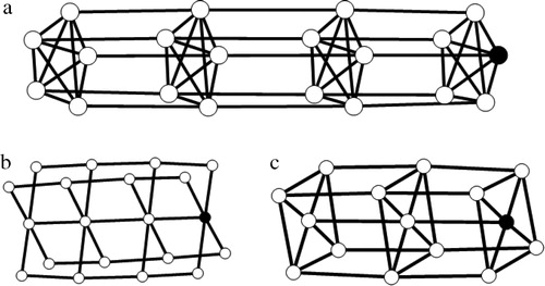
To verify the above observation, all we need to do is to select carefully a vertex that observes the entire graph. The vertex to choose for each of the respective graphs is shown in .
Remark
We can generalize Observation 2.3 and say that for ,
if the domination number of
is 1, that is
.
Observation 2.4
if
is one of the following:
(i) , where
;
(ii) , where
;
(iii) , where
and
.
Observation 2.4 can be shown by noting that no singleton can form a PDS of , and the results follow by selecting two vertices carefully as shown in .
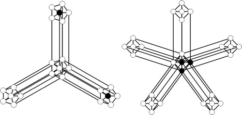
Theorem 2.5
For ,
.
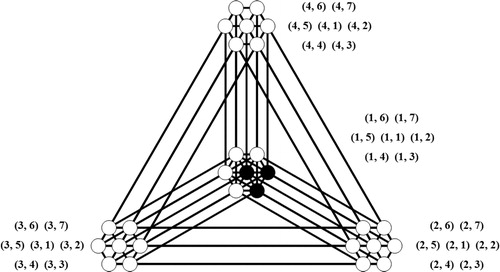
Proof
We label the vertices of as
, where
is connected to all the other vertices of an
-cycle. Similarly, we label the vertices of
as
, where
is connected to all the other vertices of an
-cycle. By the definition of the Cartesian product of two graphs, the vertices of
can be labeled as
, where
and
(see ). For simplicity, we write
to denote
. It can be verified that
is a PDS for
. □
Theorem 2.6
For ,
.
Proof
Result follows after selecting three vertices carefully as shown in . □
Theorem 2.7
For ,
(i) ;
(ii) , where
.
Proof
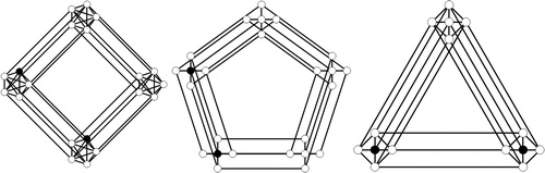
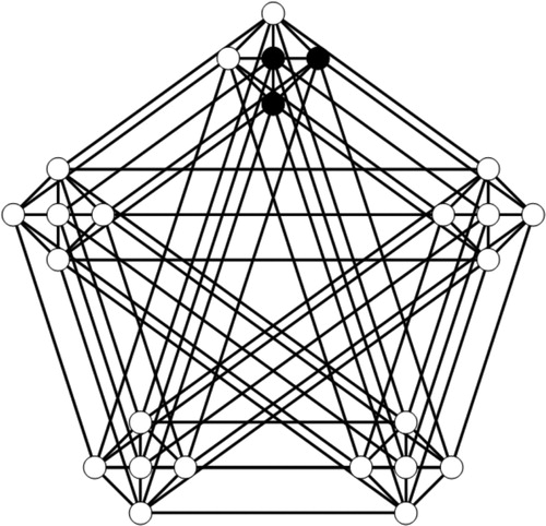
(i) Result follows after by checking that no singleton can form a PDS of , and verifying that the two vertices as shown in (left) are a PDS.
(ii) Result follows after selecting three vertices carefully as shown in (right). □
Remark
Indeed, it could be shown by exhaustion that the power domination numbers in Theorems 2.5Theorem 2.6–2.7(ii) can never be two. Thus for , we have: (a)
; (b)
; (c)
.
In the following proof for Theorem 2.8, we shall label the vertices of as
,
,
, …,
, where
is adjacent to all the end-vertices
,
, …,
. Similarly, we shall label the vertices of
as
,
,
, …,
, where
is adjacent to all the end-vertices
,
, …,
. By the definition of the Cartesian product of two graphs, the vertices of
can be labeled as
, where
and
(see ). For simplicity, we write
to denote
.
Theorem 2.8
For ,
.
Proof
We shall prove this result by induction on . When
, we can show that
for any integer
, by checking that no vertex singly observes the entire graph and verifying that
is a PDS of
. Assume that the result is true for
, that is
, where
. Noting that
, we want to show that the result holds for
, that is
.
Suppose on the contrary that . Let
be a PDS of
with cardinality
. Denote
and
.
Claim 1
There exists such that
.
To verify that our claim is true, we observe that if , then
is also a PDS for any vertex
. Furthermore, if both
and
are non-zero, then the degree of
is two. Hence result follows by Observation 1.2.
Claim 2
.
If Claim 2 is false, then it follows from Claim 1 that . By Algorithm 1.1, since
, it follows that
is adjacent to at least two unobserved vertices in
. Hence
does not observe the graph, which is a contradiction.
We are now ready to prove the inductive step. By symmetry of the graph and Claim 2, WLOG we let . Consider the graph obtained by deleting from
vertices
. The resulting graph is
, and it follows from Algorithm 1.1 that
is a PDS for
with cardinality
. This contradicts our inductive hypothesis. Hence
, which completes our proof by induction. □
The power domination number of the Cartesian product of two complete graphs is found in Soh and Koh [Citation4]. In that paper, they proved Theorem 2.9 to show that the power domination numbers of diameter two graphs can be arbitrarily large. This is in contrast with the result obtained by Zhao and Kang [Citation5] that any planar graph of diameter two has power domination number at most two.
Theorem 2.9
[Citation4]
For ,
.
In Barrera and Ferrero [Citation6], upper bounds for the power domination number of cylinders and tori
were provided.
Theorem 2.10
[Citation6]
The power domination number for the graph , where
, is
Theorem 2.11
[Citation6]
The power domination number for the graph , where
, is
The problem of determining the power domination number for was first studied in [Citation7]. In that paper, the authors found the following closed formula for
.
Theorem 2.12
[Citation7]
For the graph where
,
Let denote the
-dimensional hypercube, which is defined as
Dean et al. [Citation8] gave a lower bound and upper bound of . Pai and Chiu [Citation9] evaluated the power domination numbers for
, where
. We present their results as follows.
Theorem 2.13
[Citation8]
For the -dimensional hypercube,
Theorem 2.14
[Citation9]
For the -dimensional hypercube,
3 Vizing-like inequality
In 1968, Vizing [Citation10] proposed the following famous inequality: To date, the inequality still remains a conjecture. We conjecture that the following Vizing-like inequality holds when the power domination number is used instead.
We begin this section by giving a few definitions leading to a result on the power domination of trees. After that, we will prove that the above inequality is valid if either
or
is a tree.
A spider is a tree with at most one vertex having degree 3 or more. The spider number of a tree , denoted by
, is the minimum number of subsets into which
can be partitioned so that each subset induces a spider. We call such a partition a spider partition and each set of the partition a spider subset.
Theorem 3.15
[Citation3]
For any tree T, .
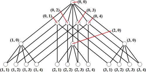
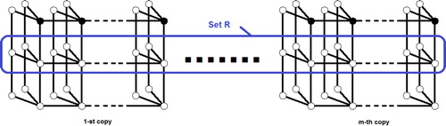
Lemma 3.16
For any connected graphs and
,
.
Proof
Let be any
vertices from
, where
. We know that at least one of the
possible combinations of
observes
. From the definition of Cartesian product, the graph
can be constructed by using
copies of
. Denote the copies as
, where
. Each vertex in
is labeled as
, where
(see ).
Consider a modified form of Algorithm 1.1 starting from some .
| 1. | (Domination) Set | ||||
| 2. | (Propagation) As long as there exists | ||||
| 3. | (Extended Propagation) If | ||||
Theorem 3.17
For any graph G and any tree T, .
Proof
Let be a PDS for the graph
,
, and
. By Theorem 3.15, we can partition
into
spider subsets
. Let
, the subgraph induced by
, where
. By Lemma 3.16,
. It follows that
, and therefore
□
Example
Consider the graph , where
. By Theorem 2.9, we have
.
4 An illustration of the Vizing-like inequality
We define the corona of two graphs and
to be the graph formed from one copy of
and
copies of
, where the
th vertex of
is adjacent to every vertex in the
th copy of
. Such graphs are denoted as
. Generally, the two graphs
and
are not isomorphic.
In this section, we are interested in finding the power domination number of the graph . Before we prove this result, we define the following and make an observation. Suppose vertex
with
. If
is adjacent with two or more end-vertices, then
is called a strong support vertex.
Observation 4.18
If has
strong support vertices, then
.
We first consider the following special case.
Lemma 4.19
For not both equal 1,
.
Proof
WLOG, we assume . When
,
. When
, since there are
strong support vertices in
, by Observation 4.18
. Then by Theorem 3.17, for
not both equal 1,
.
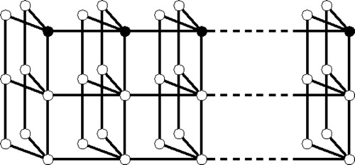
It remains to show that . When
, it can be verified that our choice of power dominating set of cardinality
as shown in observes the graph
.
When , notice that the graph
contains
copies of
with additional edges, where these additional edges are confined within the set of vertices
(see ).
We now verify that our choice of power dominating set of cardinality as shown in observes the graph
. Notice that all vertices in the set
are observed, which implies all edges in
are observed. Since each vertex in
has exactly one neighboring vertex that is unobserved, it follows that the graph is observed by our choice of power dominating set. □
Theorem 4.20
For ,
.
Proof
When , we observe that
can be observed by one vertex. So
. When
are not both equal 1, Lemma 4.19 gives the desired result. □
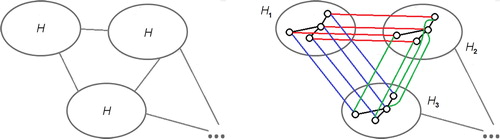
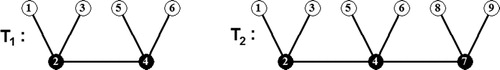
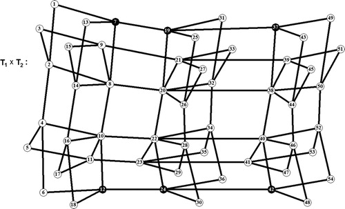
Example
Let and
be the trees as shown in . The graph of
along with its power dominating set is shown in . Notice that equality may hold for the Vizing-like inequality; for this example,
.
We would like to end this paper by proposing the following problems for further study.
Problem 1
Prove or disprove: For ,
.
Problem 2
Study the power domination problem for the graph , where
, is one of the following graphs:
or
.
Problem 3
For , construct bounds for the power domination number of the graph
Notes
Peer review under responsibility of Kalasalingam University.
References
- L. Mili, T.L. Baldwin, A.G. Phadke, Phasor measurements for voltage and transient stability monitoring and control, in: Proceedings of the EPRI-NSF Workshop on Application of Advanced Mathematics to Power Systems, San Francisco, CA, 1991.
- P.DorbecM.MollardS.KlavzarS.SpacapanPower domination in product graphsSIAM J. Discrete Math.2222008554567
- T.W.HaynesS.M.HedetniemiS.T.HedetniemiM.A.HenningDomination in graphs applied to electric power networksSIAM J. Discrete Math.1542002519529
- K.W.SohK.M.KohA note on power domination problem in diameter two graphsAKCE Int. J. Graphs Comb.11120145155
- M.ZhaoL.Y.KangPower domination in planar graphs with small diameterJ. Shanghai Univ.1132007218222
- R.BarreraD.FerreroPower domination in cylinders, tori, and generalized Petersen graphsNetworks58120114349
- M.DorflingM.A.HenningA note on power domination in grid graphsDiscrete Appl. Math.154200610231027
- N.DeanA.IlicI.RamirezJ.ShenK.TianOn the power dominating sets of hypercubesIEEE 14th International Conference on Computational Science and Engineering2011488491
- K.-J. Pai, W.-J. Chiu, A note on “on the power dominating sets of hypercubes”, in: 29th Workshop on Combinatorial Mathematics and Computation Theory, Taipei, 56, 2012.
- V.G.VizingSome unsolved problems in graph theoryUspehi Mat. Naukno.2361968117134