Construction of an α-labeled tree from a given set of α-labeled trees

Peer review under responsibility of Kalasalingam University.

Abstract

Inspired by the method of Koh et al. (1979) of combining known graceful trees to construct bigger graceful trees, a new class of graceful trees is constructed from a set of $k$ known graceful trees, $k\ge 2$ in a specific way. In fact, each member of this new class of trees admits $\alpha$-labeling, a stronger version of graceful labeling. Consequently, each member of this family of trees decomposes complete graphs and complete bipartite graphs.

Keywords:

• Graceful tree
• Graceful tree conjecture
• Graceful labeling

1 Introduction

All the graphs considered in this paper are finite simple graphs. Terms that are not defined here can be referred from the book [1]. At the Smolenice symposium in 1963, Ringel [2] conjectured that $K_{2n+1}$, the complete graph on $2n+1$ vertices, can be decomposed into $2n+1$ isomorphic copies of a given tree with $n$ edges. In 1965, Kotzig [3] also conjectured that the complete graph $K_{2n+1}$ can be cyclically decomposed into $2n+1$ copies of a given tree with $n$ edges. In an attempt to settle these two conjectures, in 1967, in his classical paper [4] Rosa introduced a hierarchical series of ‘valuations’ of a graph called $\rho ,\sigma ,\beta ,\alpha$-valuations and used these valuations to investigate the cyclic decomposition of complete graphs. Later, the $\beta$-valuation was called graceful by Golomb [5], and this term is being widely used. A function $f$ is called graceful labeling of a graph $G$ with $m$ edges, if $f$ is an injective function from $V\left(G\right)$ to $\{0,1,2,\dots ,m\}$ such that, when every edge $uv$ is assigned the edge label $|f\left(u\right)-f\left(v\right)|$, then the resulting edge labels are distinct. A graph which admits graceful labeling is called a graceful graph. A graceful labeling $f$ of a graph $G$ with $q$ edges is said to be an $\alpha$-labeling if there exists a $\lambda$ such that $f\left(u\right)\le \lambda <f\left(v\right)$ or $f\left(v\right)\le \lambda <f\left(u\right)$ for every edge $uv\in E\left(G\right)$, where $\lambda$ is called the width of the $\alpha$-labeling. It follows from the definition of $\alpha$-labeling, that if a graph $G$ has an $\alpha$-labeling $f$ with width $\lambda$, then $V_1=\{x\in V\left(G\right)|f\left(x\right)\le \lambda \}$ and $V_2=\{y\in V\left(G\right)|f\left(y\right)>\lambda \}$ form a bipartition $(V_1,V_2)$ of $V\left(G\right)$. Thus, every $\alpha$-labeled graph must be a bipartite graph. Rosa [4] also proved the following significant theorem.

Fig. 8 Renaming of vertices of tree $\hat{T}$ as defined in step 3 of Algorithm for combining $\alpha$-labeled trees $T_1,T_2$ and $T_3$.

Fig. 9 $\alpha$-labeled tree $\hat{T}$ with 58 edges.

Theorem 1

Rosa [4]

If a graph $T$ with $n$ edges has a graceful labeling, then $K_{2n+1}$ can be cyclically decomposed into $2n+1$ copies of $T$.

This result led to the Rosa–Kotzig–Ringel Conjecture popularly called Graceful Tree Conjecture, which states that “All trees are graceful”. The graceful tree conjecture has been the focus of many papers for over four decades. So far, no proof of the truth or falsity of the conjecture has been found. In the absence of a generic proof, one approach used in investigating the Graceful Tree Conjecture is proving the gracefulness of specialized classes of trees. Aldred and Mckay [6] used computer search to prove that all trees on at most 27 vertices are graceful. Michael Horton [7] has verified that all trees with at most 29 vertices are graceful. Fang [8] has verified that all trees with at most 35 vertices are graceful. Rosa [4] has proved that all paths and caterpillars are graceful. Some special classes of lobsters were shown to be graceful by Ng [9] and Wang et al. [10]. Chen, Lu and Yeh [11] have shown that all firecrackers are graceful. Sethuraman and Jeba Jesintha [12] have shown that all banana trees are graceful. Pastel and Raynaud [13] have shown that olive trees are graceful. Bermond and Sotteau [14] have proved that all symmetrical trees are graceful. One of the general results proved on Graceful Tree Conjecture is the result due to Hrnčiar et al. [15] that all trees of diameter five are graceful. Using Hrnčiar’s branch moving technique, Balbuena et al. [16] have shown that trees having an even or quasi even degree sequence are graceful. Koh, Rogers and Tan [17] gave different methods to construct a bigger graceful tree from smaller graceful trees. Burzio and Ferrarese [18] extended the method of Koh et al. and consequently they have shown that the subdivision of every graceful tree is graceful. Cahit [19] has exhibited canonic labeling technique for proving the gracefulness of a class of rooted trees. Sethuraman and Venkatesh [20] have given a method of attaching caterpillars recursively with other caterpillars to generate graceful trees. For an exhaustive survey on Graceful Tree Conjecture, refer the excellent survey by Gallian [21], for other related results refer [22,23].

2 Main result

Here we construct an $\alpha$-labeled tree from a given set of $k$ known $\alpha$-labeled trees. First we give a special arrangement of vertices of an $\alpha$-labeled tree called top to bottom arrangement. Then we give an algorithm for combining $\alpha$-labeled trees. The top to bottom arrangement of vertices of an $\alpha$-labeled tree plays an important role in this algorithm.

Let $T$ be an $\alpha$-labeled tree with $\alpha$-labeling $\theta$ and its width $\lambda$. By the definition of $\lambda$, there exists a bipartition $(V_1,V_2)$ of the vertex set $V\left(T\right)$ with the property that for each $x\in V_1$, $\theta \left(x\right)\le \lambda$ and for each $y\in V_2$, $\theta \left(y\right)>\lambda$.

Arrange the vertices of $V_1$ with respect to the increasing order of the vertex labels of the vertices of $V_1$ such that the vertex with the least label in $V_1$ appears in the top and vertex with the largest label in $V_1$ appears in the bottom. Then arrange the vertices of $V_2$ to the right side of all the vertices of $V_1$ in the following way. Arrange the vertices of $V_2$ with respect to the decreasing order of their vertex labels such that the vertex with the largest label is in the top and the vertex with the least label of $V_2$ is in the bottom. This arrangement of vertices of an $\alpha$-labeled tree $T$ is referred to as “top to bottom arrangement” corresponding to an $\alpha$-labeling $\theta$.

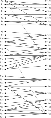
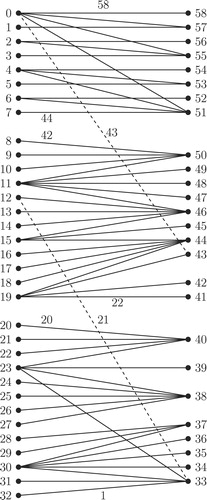
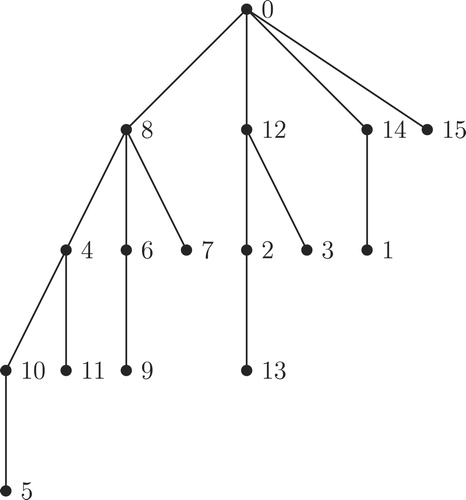
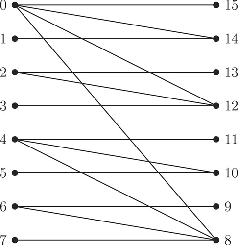
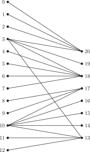
The top to bottom arrangement of an $\alpha$-labeled tree given in Fig. 1 is illustrated in Fig. 2.

Fig. 1 An $\alpha$-labeled tree $T_1$ with 15 edges.

Fig. 2 The top to bottom arrangement of vertices of $T_1$.

In the next section, we present an algorithm for combining $\alpha$-labeled trees.

2.1 Algorithm for combining $\alpha$-labeled trees

Input:

Take any set of $k$ $\alpha$-labeled trees $T_1,T_2,\dots ,T_k$ having their respective $\alpha$-labelings, ${\theta }_1,{\theta }_2,\dots ,{\theta }_k$, where $k\ge 2$, as an input. Let $m_i$ denote the number of edges of $T_i$, for $1\le i\le k$ and let ${\lambda }_i$ denote the width of the $\alpha$-labeling ${\theta }_i$ of the trees $T_i$, for $1\le i\le k$.

Step 1: Arrangement of the vertices of $T_i$’s, $1\le i\le k$

Arrange the vertices of $T_1$ in the top to bottom arrangement. Next, arrange the vertices of $T_2$ in the top to bottom arrangement below to all the vertices of $T_1$. Similarly, for $3\le i\le k$, arrange the vertices of $T_i$ in the top to bottom arrangement below to all the vertices of $T_{i-1}$.

Step 2: Addition of a new edge between $T_i$ and $T_{i+1}$, for each $i$, $1\le i\le k-1$.

Step 2.1:

If $(m_{i+1}-{\lambda }_{i+1})>({\lambda }_i+1)$, choose any one vertex, say $u\in V_1\left(T_i\right)$ having the vertex label ${\theta }_i\left(u\right)=x\in \{0,1,2,\dots ,{\lambda }_i\}$ then correspondingly find the vertex $z\in V_2\left(T_{i+1}\right)$ with vertex label ${\theta }_{i+1}\left(z\right)=(m_{i+1}-{\lambda }_i+x)$ from the tree $T_{i+1}$. Add a new edge between the vertex $u$ of $T_i$ and the vertex $z$ of $T_{i+1}$.

Step 2.2:

If $(m_{i+1}-{\lambda }_{i+1})\le ({\lambda }_i+1)$, choose any one vertex, say $v\in V_1\left(T_i\right)$ having the vertex label ${\theta }_i\left(v\right)=y\in \{{\lambda }_i+1-m_{i+1}+{\lambda }_{i+1},{\lambda }_i+1-m_{i+1}+{\lambda }_{i+1}-1,\dots ,{\lambda }_i\}$ then correspondingly find the vertex $w\in V_2\left(T_{i+1}\right)$ with vertex label ${\theta }_{i+1}\left(w\right)=(y+m_{i+1}-{\lambda }_i)$ from the tree $T_{i+1}$. Add a new edge between the vertex $v$ of $T_i$ and the vertex $w$ of $T_{i+1}$.

Call the resultant tree thus obtained as $\hat{T}$.

Step 3: Labeling of the Vertices of $\hat{T}$

Arrange the vertices of $V_1\left(T_1\right)$ as a sequence as appears in the top to bottom arrangement corresponding to the $\alpha$-labeling ${\theta }_1$.

Then, for $2\le i\le k$, arrange the vertices of $V_1\left(T_i\right)$ following the bottom most vertex of $V_1\left(T_{i-1}\right)$ as a sequence as appears in the top to bottom arrangement corresponding to the $\alpha$-labeling ${\theta }_i$. Denote this sequence of vertices of $V_1\left(T_i\right)$ for $i=1,2,\dots ,k$ (in the increasing order of index $i$) in $\hat{T}$ as $V_1\left(\hat{T}\right)$.

Arrange the vertices of $V_2\left(T_1\right)$ as a sequence as appears in the top to bottom arrangement corresponding to the $\alpha$-labeling ${\theta }_1$. Then, for $2\le i\le k$, arrange the vertices of $V_2\left(T_i\right)$ following the bottom most vertex of $V_2\left(T_{i-1}\right)$ as a sequence as appears in the top to bottom arrangement corresponding to the $\alpha$-labeling ${\theta }_i$. Denote this sequence of vertices of $V_2\left(T_i\right)$ for $i=1,2,\dots ,k$ (in the increasing order of index $i$) in $\hat{T}$ as $V_2\left(\hat{T}\right)$.

Rename the vertices of $V_1\left(\hat{T}\right)$ on the left side partition of the vertices of $\hat{T}$ as $v_0,v_1,v_2,\dots ,v_{r-1}$ in the top to bottom order, where $\left|V_1\left(\hat{T}\right)\right|=r$ and the vertices of $V_2\left(\hat{T}\right)$ on the right side partition of the vertices of $\hat{T}$ as $v_M,v_{M-1},\dots ,v_r$ in the top to bottom order.

Define $\theta :V\left(\hat{T}\right)=\{v_0,v_1,\dots ,v_M\}\to \{0,1,2,\dots ,M\}$,

by $\theta \left(v_i\right)=i$, for $i$, $0\le i\le M$.

Step 4: Edge labeling of edges of $\hat{T}$

For every edge $uv$ of $\hat{T}$, define the edge label ${\theta }^{\prime }\left(uv\right)=|\theta \left(u\right)-\theta \left(v\right)|$.

2.2 Correctness of Algorithm for combining $\alpha$-labeled trees

Here we prove the correctness of the Algorithm for combining $\alpha$-labeled trees. More precisely, we show that the tree $\hat{T}$ constructed by the above algorithm is an $\alpha$-labeled tree. To prove the correctness we give below Observations 2.1, 2.2, 2.3 and Lemma 2. Finally we give the correctness in Theorem 3.

Observation 2.1

The vertex $z$ that defined in Step 2.1 of Algorithm for combining $\alpha$-labeled trees always exists in $V_2\left(T_{i+1}\right)$ with vertex label $(m_{i+1}-{\lambda }_i+x)$, for $1\le i\le k-1$, for every choice of the vertex $u$ in $V_1\left(T_i\right)$ with vertex label ${\theta }_i\left(u\right)=x\in \{0,1,2,\dots ,{\lambda }_i\}$, whenever $(m_{i+1}-{\lambda }_{i+1})>({\lambda }_i+1)$.

Proof

Let $(m_{i+1}-{\lambda }_{i+1})>({\lambda }_i+1)$. Suppose $x=0$. Then $m_{i+1}-{\lambda }_i+x=m_{i+1}-{\lambda }_i\le m_{i+1}$, since ${\lambda }_i\ge 0$. As $(m_{i+1}-{\lambda }_{i+1})>({\lambda }_i+1)$, we have $m_{i+1}-{\lambda }_i>{\lambda }_{i+1}+1$.

Suppose $x={\lambda }_i$. Then $m_{i+1}-{\lambda }_i+x=m_{i+1}$. Since $(m_{i+1}-{\lambda }_{i+1})>({\lambda }_i+1)$, we have $m_{i+1}-{\lambda }_i>{\lambda }_{i+1}+1$. Therefore, ${\lambda }_{i+1}+1\le m_{i+1}-{\lambda }_i+x\le m_{i+1}$, for every $x\in \{0,1,2,\dots ,{\lambda }_i\}$. Since $T_{i+1}$ is an $\alpha$-labeled tree, there exists a vertex in $V_2\left(T_{i+1}\right)$ with vertex label $(m_{i+1}-{\lambda }_i+x)$. Denote the vertex of $V_2\left(T_{i+1}\right)$ with vertex label $(m_{i+1}-{\lambda }_i+x)$ as $z$. Thus, there exists a vertex $z$ in $V_2\left(T_{i+1}\right)$ with ${\theta }_{i+1}\left(z\right)=(m_{i+1}-{\lambda }_i+x)$ for any $x\in \{0,1,2,\dots ,{\lambda }_i\}$.  □

Observation 2.2

The vertex $w$ that defined in Step 2.2 of Algorithm for combining $\alpha$-labeled trees always exists in $V_2\left(T_{i+1}\right)$ with vertex label $(m_{i+1}-{\lambda }_i+y)$, for $1\le i\le k-1$, for every choice of the vertex $v$ in $V_1\left(T_i\right)$ with vertex label ${\theta }_i\left(v\right)=y\in \{{\lambda }_i+1-m_{i+1}+{\lambda }_{i+1},{\lambda }_i+1-m_{i+1}+{\lambda }_{i+1}-1\cdots ,{\lambda }_i\}$ whenever $(m_{i+1}-{\lambda }_{i+1})\le ({\lambda }_i+1)$.

Proof

Let $(m_{i+1}-{\lambda }_{i+1})\le ({\lambda }_i+1)$. Suppose $y={\lambda }_i+1-m_{i+1}+{\lambda }_{i+1}$. Then $m_{i+1}-{\lambda }_i+y={\lambda }_{i+1}+1>{\lambda }_{i+1}$. Suppose $y={\lambda }_i$. Then $m_{i+1}-{\lambda }_i+y=m_{i+1}\le m_{i+1}$. Therefore, ${\lambda }_{i+1}+1\le m_{i+1}-{\lambda }_i+y\le m_{i+1}$, for every $y\in \{{\lambda }_i+1-m_{i+1}+{\lambda }_{i+1},{\lambda }_i+1-m_{i+1}+{\lambda }_{i+1}-1\cdots ,{\lambda }_i\}$. Since $T_{i+1}$ is an $\alpha$-labeled tree, there exists a vertex in $V_2\left(T_{i+1}\right)$ with vertex label $(m_{i+1}-{\lambda }_i+y)$. Denote the vertex of $V_2\left(T_{i+1}\right)$ with vertex label $(m_{i+1}-{\lambda }_i+y)$ as $w$. Thus, there exists a vertex $w$ in $V_2\left(T_{i+1}\right)$ with ${\theta }_{i+1}\left(w\right)=(m_{i+1}-{\lambda }_i+y)$ for any $y\in \{{\lambda }_i+1-m_{i+1}+{\lambda }_{i+1},{\lambda }_i+1-m_{i+1}+{\lambda }_{i+1}-1\cdots ,{\lambda }_i\}$.  □

Observation 2.3

The output tree $\hat{T}$ obtained from the given set of trees $T_i$ having $m_i$ edges, for $1\le i\le k$ contains $M=m_1+m_2+m_3+\cdots +m_k+(k-1)$ edges. It is clear from Step 3 of Algorithm for combining $\alpha$-labeled trees that every vertex of $\hat{T}$ gets distinct vertex labels from the set $\{0,1,2,\dots ,M\}$.

Lemma 2

The edge labels of the edges of $\hat{T}$ that are defined in Step 4 of Algorithm for combining $\alpha$-labeled trees are distinct and ranges from 1 to $M$, where $M=\left|E\left(\hat{T}\right)\right|$.

Proof

Observe from Step 3 of Algorithm for combining $\alpha$-labeled trees, for a vertex $v$ of $T_i$ in $\hat{T}$, for $1\le i\le k$, we have (1) $\theta \left(v\right)=\left\{\begin{array}{cc}{\theta }_i\left(v\right)+\sum _{j=1}^{i-1}{\lambda }_j+(i-1),\hfill & \text{if}v\in V_1\left(T_i\right)\hfill \\ {\theta }_i\left(v\right)+\sum _{j=1}^k{\lambda }_j+(k-1)+\sum _{j=i+1}^k(m_j-{\lambda }_j)-{\lambda }_i,\hfill & \text{if}v\in V_2\left(T_i\right).\hfill \end{array}\right.$(1) Let $uv$ be any edge of $\hat{T}$.

Case 1: Suppose $uv\in E\left(T_i\right)$ for some i, $1\le i\le k.$

Without loss of generality, we assume that $u\in V_1\left(T_i\right)$ and $v\in V_2\left(T_i\right)$. Then, $\begin{array}{cc}{\theta }^{\prime }\left(uv\right)\hfill & =|\theta \left(u\right)-\theta \left(v\right)|\hfill \\ \hfill & =\theta \left(v\right)-\theta \left(u\right)\hfill \\ \hfill & ={\theta }_i\left(v\right)+\sum _{j=1}^k{\lambda }_j+(k-1)+\sum _{j=i+1}^k(m_j-{\lambda }_j)-{\lambda }_i-\left[{\theta }_i\left(u\right)+\sum _{j=1}^{i-1}{\lambda }_j+(i-1)\right]\hfill \\ \hfill & ={\theta }_i\left(v\right)-{\theta }_i\left(u\right)+\sum _{j=i+1}^k{\lambda }_j+(k-1)+\sum _{j=i+1}^k(m_j-{\lambda }_j)-i+1\hfill \\ \hfill & ={\theta }_i^{\prime }\left(uv\right)+\sum _{j=i+1}^k{\lambda }_j+(k-1)+\sum _{j=i+1}^k(m_j-{\lambda }_j)-i+1.\hfill \end{array}$That is, (2) ${\theta }^{\prime }\left(uv\right)={\theta }_i^{\prime }\left(uv\right)+\sum _{j=i+1}^k{\lambda }_j+(k-1)+\sum _{j=i+1}^k(m_j-{\lambda }_j)-i+1.$(2) From Eq. (2(2) ${\theta }^{\prime }\left(uv\right)={\theta }_i^{\prime }\left(uv\right)+\sum _{j=i+1}^k{\lambda }_j+(k-1)+\sum _{j=i+1}^k(m_j-{\lambda }_j)-i+1.$(2) ), one can observe that the edge label of every edge $uv$ of $T_i$ in $\hat{T}$ is translated by ${\sum }_{j=i+1}^k{\lambda }_j+(k-1)+{\sum }_{j=i+1}^k(m_j-{\lambda }_j)-i+1$ from the edge label of the edge $uv$ of $T_i$ induced by its $\alpha$-labeling ${\theta }_i$, for $i$, $1\le i\le k$.

Since ${\theta }_i$ is an $\alpha$-labeling, the edge labels of edges of $T_i$ induced by ${\theta }_i$ are distinct, for $i$, $1\le i\le k$. Therefore from the above observation, edge labels of the edges of $T_i$ are distinct whenever the edges are in $E\left(T_i\right)$ for some $i$, $1\le i\le k$.

From Eq. (2(2) ${\theta }^{\prime }\left(uv\right)={\theta }_i^{\prime }\left(uv\right)+\sum _{j=i+1}^k{\lambda }_j+(k-1)+\sum _{j=i+1}^k(m_j-{\lambda }_j)-i+1.$(2) ), the maximum of all the edge labels of edges of $T_{i+1}$ in $\hat{T}$, for $i$, $1\le i\le k-1$ is $m_{i+1}+\sum _{j=i+2}^k{\lambda }_j+(k-1)+\sum _{j=i+2}^k(m_j-{\lambda }_j)-(i+1)+1.$The minimum of all the edge labels of edges of $T_i$ in $\hat{T}$ for $1\le i\le k$ is $1+\sum _{j=i+1}^k{\lambda }_j+(k-1)+\sum _{j=i+1}^k(m_j-{\lambda }_j)-i+1.$

Then, for $i$, $1\le i\le k-1$,

$\left[1+\sum _{j=i+1}^k{\lambda }_j+(k-1)+\sum _{j=i+1}^k(m_j-{\lambda }_j)-i+1\right]$$-\left[m_{i+1}+\sum _{j=i+2}^k{\lambda }_j+(k-1)+\sum _{j=i+2}^k(m_j-{\lambda }_j)-(i+1)+1\right]=2.$

Therefore, minimum of all the edge labels of edges of $T_i$ in $\hat{T}$ is greater than the maximum of all the edge labels of $T_{i+1}$ in $\hat{T}$, for $i$, $1\le i\le k-1$. Thus, the edge labels of edges of $T_i$ and the edge labels of edges of $T_{i+1}$ do not over lap. Hence, edge labels of the edges of $T_i$ and that of $T_j$ do not over lap for any $i,j$, $1\le i<j\le k$.

Claim 1

For each $i$, $1\le i\le k-1$, the edge label of the new edge added between a vertex in $V_1\left(T_i\right)$ and a vertex in $V_2\left(T_{i+1}\right)$ by Step 2 of Algorithm is ${\sum }_{j=i+1}^k{\lambda }_j+(k-1)+{\sum }_{j=i+1}^k(m_j-{\lambda }_j)-i+1.$

Observe from Step 2 of Algorithm for combining $\alpha$-labeled trees, a new edge is added between $T_i$ and $T_{i+1}$ for each $i$, $1\le i\le k-1$ to obtain the tree $\hat{T}$. The addition of the new edge is done in two cases depending on $(m_{i+1}-{\lambda }_{i+1})>({\lambda }_i+1)$ or $(m_{i+1}-{\lambda }_{i+1})\le ({\lambda }_i+1)$.

Case 2.1: When $(m_{i+1}-{\lambda }_{i+1})>({\lambda }_i+1)$.

Then the new edge is added between a vertex $u$ of $T_i$ with vertex label ${\theta }_i\left(u\right)=x\in \{0,1,2,\dots ,{\lambda }_i\}$ and the vertex $z$ of $T_{i+1}$ with vertex label ${\theta }_{i+1}\left(z\right)=(m_{i+1}-{\lambda }_i+x)$.

Since $u\in V_1\left(T_i\right)$, by Eq. (1(1) $\theta \left(v\right)=\left\{\begin{array}{cc}{\theta }_i\left(v\right)+\sum _{j=1}^{i-1}{\lambda }_j+(i-1),\hfill & \text{if}v\in V_1\left(T_i\right)\hfill \\ {\theta }_i\left(v\right)+\sum _{j=1}^k{\lambda }_j+(k-1)+\sum _{j=i+1}^k(m_j-{\lambda }_j)-{\lambda }_i,\hfill & \text{if}v\in V_2\left(T_i\right).\hfill \end{array}\right.$(1) ) we have, $\begin{array}{cc}\theta \left(u\right)\hfill & ={\theta }_i\left(u\right)+\sum _{j=1}^{i-1}{\lambda }_j+(i-1)\hfill \\ \hfill & =x+\sum _{j=1}^{i-1}{\lambda }_j+(i-1),\text{where}x\in \{0,1,2,\dots ,{\lambda }_j\}.\hfill \end{array}$Since $z\in V_2\left(T_{i+1}\right)$, by Eq. (1(1) $\theta \left(v\right)=\left\{\begin{array}{cc}{\theta }_i\left(v\right)+\sum _{j=1}^{i-1}{\lambda }_j+(i-1),\hfill & \text{if}v\in V_1\left(T_i\right)\hfill \\ {\theta }_i\left(v\right)+\sum _{j=1}^k{\lambda }_j+(k-1)+\sum _{j=i+1}^k(m_j-{\lambda }_j)-{\lambda }_i,\hfill & \text{if}v\in V_2\left(T_i\right).\hfill \end{array}\right.$(1) ) we have, $\begin{array}{cc}\theta \left(z\right)\hfill & ={\theta }_{i+1}\left(z\right)+\sum _{j=1}^k{\lambda }_j+(k-1)+\sum _{j=i+2}^k(m_j-{\lambda }_j)-{\lambda }_{i+1}\hfill \\ \hfill & =(m_{i+1}-{\lambda }_i+x)+\sum _{j=1}^k{\lambda }_j+(k-1)+\sum _{j=i+2}^k(m_j-{\lambda }_j)-{\lambda }_{i+1}.\hfill \end{array}$Therefore, the edge label of the new edge $uz$ in $\hat{T}$ is ${\theta }^{\prime }\left(uz\right)=|\theta \left(u\right)-\theta \left(z\right)|=\theta \left(z\right)-\theta \left(u\right)=\left[(m_{i+1}-{\lambda }_i+x)+\sum _{j=1}^k{\lambda }_j+(k-1)+\sum _{j=i+2}^k(m_j-{\lambda }_j)-{\lambda }_{i+1}\right]-\left[x+\sum _{j=1}^{i-1}{\lambda }_j+(i-1)\right]=m_{i+1}-{\lambda }_i+x+\sum _{j=i}^k{\lambda }_j+(k-1)+\sum _{j=i+2}^k(m_j-{\lambda }_j)-{\lambda }_{i+1}-x-i+1=\sum _{j=i+1}^k{\lambda }_j+(k-1)+\sum _{j=i+1}^k(m_j-{\lambda }_j)-i+1.$Hence the claim for the case.

Case 2.2: When $(m_{i+1}-{\lambda }_{i+1})\le ({\lambda }_i+1)$.

Then the new edge is added between a vertex $v$ of $T_i$ with vertex label ${\theta }_i\left(v\right)=y\in \{{\lambda }_i+1-m_{i+1}+{\lambda }_{i+1},{\lambda }_i+1-m_{i+1}+{\lambda }_{i+1}-1\cdots ,{\lambda }_i\}$ and the vertex $w$ of $T_{i+1}$ with vertex label ${\theta }_{i+1}\left(w\right)=(m_{i+1}-{\lambda }_i+y)$.

Since $v\in V_1\left(T_i\right)$, by Eq. (1(1) $\theta \left(v\right)=\left\{\begin{array}{cc}{\theta }_i\left(v\right)+\sum _{j=1}^{i-1}{\lambda }_j+(i-1),\hfill & \text{if}v\in V_1\left(T_i\right)\hfill \\ {\theta }_i\left(v\right)+\sum _{j=1}^k{\lambda }_j+(k-1)+\sum _{j=i+1}^k(m_j-{\lambda }_j)-{\lambda }_i,\hfill & \text{if}v\in V_2\left(T_i\right).\hfill \end{array}\right.$(1) ) we have, $\begin{array}{cc}\theta \left(v\right)\hfill & ={\theta }_i\left(v\right)+\sum _{j=1}^{i-1}{\lambda }_j+(i-1)\hfill \\ \hfill & =y+\sum _{j=1}^{i-1}{\lambda }_j+(i-1),\hfill \\ \hfill & \text{where}y\in \{{\lambda }_i+1-m_{i+1}+{\lambda }_{i+1},{\lambda }_i+1-m_{i+1}+{\lambda }_{i+1}-1\cdots ,{\lambda }_i\}.\hfill \end{array}$Since $w\in V_2\left(T_{i+1}\right)$, by Eq. (1(1) $\theta \left(v\right)=\left\{\begin{array}{cc}{\theta }_i\left(v\right)+\sum _{j=1}^{i-1}{\lambda }_j+(i-1),\hfill & \text{if}v\in V_1\left(T_i\right)\hfill \\ {\theta }_i\left(v\right)+\sum _{j=1}^k{\lambda }_j+(k-1)+\sum _{j=i+1}^k(m_j-{\lambda }_j)-{\lambda }_i,\hfill & \text{if}v\in V_2\left(T_i\right).\hfill \end{array}\right.$(1) ) we have, $\begin{array}{cc}\theta \left(w\right)\hfill & ={\theta }_{i+1}\left(w\right)+\sum _{j=1}^k{\lambda }_j+(k-1)+\sum _{j=i+2}^k(m_j-{\lambda }_j)-{\lambda }_{i+1}\hfill \\ \hfill & =(m_{i+1}-{\lambda }_i+y)+\sum _{j=1}^k{\lambda }_j+(k-1)+\sum _{j=i+2}^k(m_j-{\lambda }_j)-{\lambda }_{i+1}.\hfill \end{array}$Therefore, the edge label of the new edge $vw$ in $\hat{T}$ is ${\theta }^{\prime }\left(vw\right)=|\theta \left(v\right)-\theta \left(w\right)|=\theta \left(w\right)-\theta \left(v\right)=\left[(m_{i+1}-{\lambda }_i+y)+\sum _{j=1}^k{\lambda }_j+(k-1)+\sum _{j=i+2}^k(m_j-{\lambda }_j)-{\lambda }_{i+1}\right]-\left[y+\sum _{j=1}^{i-1}{\lambda }_j+(i-1)\right]=m_{i+1}-{\lambda }_i+y+\sum _{j=i}^k{\lambda }_j+(k-1)+\sum _{j=i+2}^k(m_j-{\lambda }_j)-{\lambda }_{i+1}-y-i+1=\sum _{j=i+1}^k{\lambda }_j+(k-1)+\sum _{j=i+1}^k(m_j-{\lambda }_j)-i+1.$Hence the claim for the case.

Therefore,

Edge label of the new edge added between $T_i$ and $T_{i+1}$

$=$ (minimum edge label of $T_i$) $-$ 1

$=$ (maximum edge label of $T_{i+1}$) $+$ 1, for all $i$, $1\le i\le k-1$.

As a consequence the edge labels of all the edges of $\hat{T}$ are distinct and hence they can be arranged as a sequence $1,2,3,\dots ,M$, where $M=\left|E\left(\hat{T}\right)\right|$.  □

Theorem 3

The output labeled tree $\hat{T}$ obtained from Algorithm for combining $\alpha$-labeled trees is an $\alpha$-labeled tree.

Proof

From Observation 2.3, it is clear that the vertex labels of the vertices of $\hat{T}$ that are defined in Step 3 of Algorithm for combining $\alpha$-labeled trees are distinct and the vertex labels of $M+1$ vertices of $\hat{T}$ are defined from the set $\{0,1,2,\dots ,M\}$. Also from Lemma 2, the edge labels of the $M$ edges of $\hat{T}$ are distinct and are defined from the set $\{1,2,3,\dots ,M\}$. Thus $\hat{T}$ is graceful. Further from Eq. (1(1) $\theta \left(v\right)=\left\{\begin{array}{cc}{\theta }_i\left(v\right)+\sum _{j=1}^{i-1}{\lambda }_j+(i-1),\hfill & \text{if}v\in V_1\left(T_i\right)\hfill \\ {\theta }_i\left(v\right)+\sum _{j=1}^k{\lambda }_j+(k-1)+\sum _{j=i+1}^k(m_j-{\lambda }_j)-{\lambda }_i,\hfill & \text{if}v\in V_2\left(T_i\right).\hfill \end{array}\right.$(1) ), it follows that the vertex label of any vertex in $V_1\left(\hat{T}\right)$ is less than or equal to ${\sum }_{j=1}^k{\lambda }_j+(k-1)$ and the vertex label of any vertex in $V_2\left(\hat{T}\right)$ is greater than ${\sum }_{j=1}^k{\lambda }_j+(k-1)$. Therefore, the output labeled tree $\hat{T}$ is an $\alpha$-labeled tree with the width ${\sum }_{j=1}^k{\lambda }_j+(k-1)$.  □

Since the output labeled tree $\hat{T}$ of Algorithm for combining $\alpha$-labeled trees admits $\alpha$-labeling, the following corollary is a direct consequence of Theorems 1 and 3.

Corollary 3.1

The complete graph $K_{2cq+1}$ and the complete bipartite graph $K_{mq,nq}$ can be decomposed into isomorphic copies of the $\alpha$-labeled tree $\hat{T}$, the output tree of Algorithm for combining $\alpha$-labeled trees from the input $\alpha$-labeled trees $T_1,T_2,\dots ,T_k$, where $k\ge 1$ and $m,n,c$ are arbitrary positive integers.

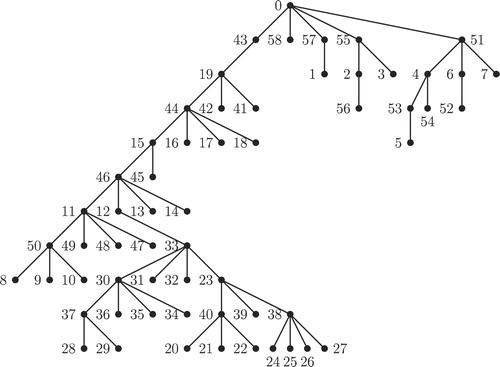
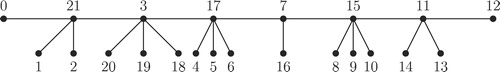
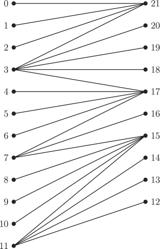
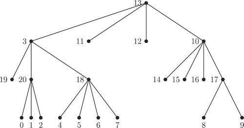
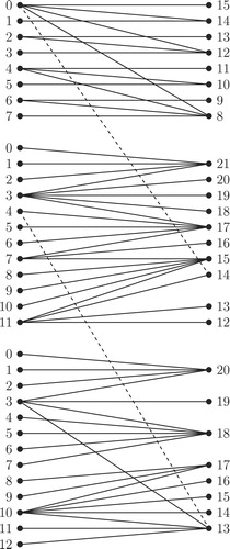
Illustrative example for Algorithm for combining $\alpha$-labeled trees

The process of Algorithm for combining $\alpha$-labeled trees is illustrated in Fig. 1 through Fig. 10. Figs. 2, 4 and 6 illustrate the top to bottom arrangement of the trees given in Figs. 1, 3 and 5 respectively. Addition of new edges as defined in Step 2 of Algorithm for combining $\alpha$-labeled trees is illustrated in Fig. 7. The output tree $\hat{T}$ of Algorithm for combining $\alpha$-labeled trees for the input trees given in Figs. 1, 3 and 5 is given in Fig. 10.

Fig. 10 The output $\alpha$-labeled tree $\hat{T}$ obtained by Algorithm for combining $\alpha$-labeled trees.

Fig. 3 An $\alpha$-labeled tree $T_2$ with 21 edges.

Fig. 4 The top to bottom arrangement of vertices of $T_2$.

Fig. 5 An $\alpha$-labeled tree $T_3$ with 20 edges.

Fig. 6 The top to bottom arrangement of vertices of $T_3$.

Fig. 7 Addition of new edges as defined in Step 2 of Algorithm for combining $\alpha$-labeled trees $T_1,T_2$ and $T_3$.

Notes

Peer review under responsibility of Kalasalingam University.

References

- West D.B. Introduction to Graph Theory second ed. 2001 Prentice Hall of India
- Ringel G. Problem 25 Theory of Graphs and Its Applications Proc. Symposium Smolenice, Prague (1963) 162.
- Kotzig A. Decompositions of a complete graph into 4k-gons Matematicky Casopis 15 1965 229 233 (in Russian)
- Rosa A. On certain valuations of the vertices of a graph Theory of Graphs, International Symposium, Rome, July 1966 1967 Gordon and Breach N.Y. and Dunod Paris 349 355
- Golomb S.W. How to number a graph Read R.C. Graph Theory and Computing 1972 Academic Press New York 23 37
- Aldred R.E. Mckay B.D. Graceful and harmonious labelings of trees Bull. Inst. Combin. Appl. 23 1998 69 72
- Michael Horton, Graceful Trees Statistics and Algorithms (Master’s thesis), http://eprints.comp.utas.edu.au:81/archieve/00000019/01/
- W. Fang, A computational approach to the graceful tree conjecture, http://arxiv:1003.3045v1[cs.DM]
- Ng H.K. Gracefulness of a class of lobsters Notices Amer. Math. Soc. 7 1986 825-05-294
- Wang J.G. Jin D.J. Lu X.G. Zhang D. The gracefulness of a class of lobster trees Math. Comput. Modelling 20 1994 105 110
- W.C. Chen, H.I. Lu, Y.N. Yeh, Operations of interlaced trees and graceful trees, Southeast Asian Bull. Math. 21 337–348
- Jeba Jesintha J. Sethuraman G. All arbitrary fixed generalized banana trees are graceful Math. Comput. Sci. 5 2011 1, 51 62
- Pastel A.M. Raynaud H. Numerotation gracieuse des olivers Colloq. Grenoble 1978 Publications Universite de Grenoble 218 223
- Bermond J.C. Sotteau D. Graph decompositions and G-design Proc. 5th British Combin. Conf., 53–72 (second series), vol. 12 1989 25 28
- Hrnčiar P. Haviar A. All trees of diameter five are graceful Discrete Math. 233 2001 133 150
- Balbuena C. Garcia-Vazquez P. Marcote X Valenzuela J.C. Trees having an even or quasi even degree sequence are graceful Appl. Math. Lett. 20 2007 370 375
- Koh K.H. Rogers D.G. Tan T. Two theorems on graceful trees Discrete Math. 25 1979 141 148
- Burzio M. Ferrarese G. The subdivision graph of a graceful tree is a graceful tree Discrete Math. 181 1998 275 281
- I. Cahit, Graceful labelings of rooted complete trees, 2002, preprint
- Sethuraman G. Venkatesh S. Decomposition of complete graphs and complete bipartite graphs into α-labeled trees Ars Combin. 93 2009 371 385
- Gallian J.A. A dynamic survey of graph labeling Electron. J. Combin. 18 2015 #DS6
- Van Bussel F. Relaxed graceful labelings of trees Electron. J. Combin. 9 2002 #R4
- Slater P.J. On k-graceful graphs Proc. of the 13th S.E. Conf. on Combinatorics, Graph Theory and Computing 1982 53 57