
 ?Mathematical formulae have been encoded as MathML and are displayed in this HTML version using MathJax in order to improve their display. Uncheck the box to turn MathJax off. This feature requires Javascript. Click on a formula to zoom.
Abstract
Let be the set of all
matrices, where
and
are the sums of entries in row
and column
, respectively. Sampling efficiently uniformly at random elements of
is a problem with interesting applications in Combinatorics and Statistics. To calibrate the statistic
for testing independence, Diaconis and Gangolli proposed a Markov chain on
that samples uniformly at random contingency tables of fixed row and column sums. Although the scheme works well for practical purposes, no formal proof is available on its rate of convergence. By using a canonical path argument, we prove that this Markov chain is fast mixing and the mixing time
is given by
where
is the maximal value in a cell.
1 Introduction
An contingency table is an
array where the sum of entries in row
is
and the sum of entries in column
is
. Let the size of a contingency table be the multiset of its rows and columns sums
and
. The combinatorial problems involving contingency tables are varied and interesting. They include counting magic squares and enumerating permutations by descent patterns and counting double cosets of symmetric groups. Contingency tables are also useful in the study of induced representations, tensor products and symmetric functions. See [Citation1] for a comprehensive introduction on these topics. Moreover, random sampling contingency tables is a problem that has statistical applications, as illustrated in [Citation2,Citation3]. For graph theoretic concepts, we refer to [Citation4].
While entries in contingency tables may be any non-negative integers, the case where entries are or
had deserved a special attention in the literature [1–3,5–12Citation[1]Citation[2]Citation[3]Citation[5]Citation[6]Citation[7]Citation[8]Citation[9]Citation[10]Citation[11]Citation[12]]. Indeed,
matrices are much researched upon for its relevance in various fields of sciences, such as network modeling in ecology, social sciences, chemical compounds and biochemical networks in the cell, where they serve to model bipartite graphs with fixed degree sequences. Although random sampling contingency tables and
matrices problems seem similar, the present paper focuses exclusively on the former.
Let be the set of
contingency tables. One way to sample a table at random is to construct a random walk that starts at a given element of
, then moves to another element according to some simple rule which changes one element to another. After
steps, one outputs the element reached by the random walk and considers this element, the
th state reached, as a random sample. Such a random walk is a Markov chain.
Although this description seems straightforward, there are two issues at stake. First of all, the rule of transition describing the local perturbation from one element to another has to be simple enough so that it can be implemented. Moreover, the local perturbation must be such that, starting from any element, any other element has a chance to be visited. If the Markov chain is viewed as a random walk on a digraph so that the elements of
are vertices of
, the last condition is equivalent to require that
be strongly connected. In [Citation1,Citation2], the following Markov chain is proposed. Take an
contingency table
where entries in row
add up to
and entries in column
add up to
. Choose at random two rows
and
and two columns
and
. Then make the following local perturbation on table
, changing it into the array
by the rule
,
,
, and
. Move from
to
if
has no negative entry, and stay on
otherwise. It can be easily proved that this operation is a local perturbation that defines a random walk which visits all the contingency tables having row sums and column sums
and
, respectively.
There is another issue to be addressed which is as follows. Since the successive states of a Markov chain are not independent, an unbiased sample can only be obtained if the chain reaches stationarity, the stage when the probability of sampling a particular configuration is fixed in time. The mixing time of a Markov chain is the number of steps required to reach that stationary state up to a defined . The information about the mixing time of a particular Markov chain is important to avoid to get a biased sample (if stationarity is not reached), or to avoid the computational cost of running the chain more than necessary. The present paper solves this problem by showing that the Markov chain proposed in [Citation1,Citation2,Citation13] mixes fast. That is, the stationary state is reached after a number of steps which is polynomial on
, the size of the contingency table having fixed row and column sums
and
, respectively. For the closely related problem of sampling
matrices, some partial results are available. Indeed, while the mixing time of the general problem is still an open problem, it had been proven by Erdos et al. [Citation14] to be fast mixing for semi-regular degree sequences only.
2 Basics on Markov chains
Let be a Markov chain on a set of states
. Let
be the matrix of transitions from one state to another. One may visualize the Markov chain
as a weighted directed graph
, where the states are the vertices of
and there is an edge of weight
if the transition from state
to state
has probability
. A Markov chain is irreducible if for all pairs of states
and
, there is an integer
, depending on the pair
, such that
. In terms of the digraph
, the Markov chain is irreducible if there is a directed path between every pair of vertices of
. A Markov chain is aperiodic if for all states
, there is an integer
such that for all
,
. That is, after sufficient number of iterations, the chain has a positive probability to stay on
at every subsequent step. This ensures that the return to state
is not periodic. In terms of the graph
, this can be achieved by having a loop at every vertex. A Markov chain is ergodic if it is irreducible and aperiodic. If
is the matrix of transitions of an ergodic Markov chain, it can be shown that there is an integer
such that for all the pairs of states
,
. (Notice that
does not depend on the pair). Also, it can be proven that for every ergodic Markov chain with transition matrix
, the largest eigenvalue of
only occurs once and is equal to 1 (Perron–Frobenius Theorem). Using this, it can be proved that there is a unique probability vector
, such that
. The vector
is the stationary distribution of
. A chain is reversible if
for every pair of states
and
. If a chain is reversible and the matrix
is symmetric, then
for every pair
and
. The stationary state is then said to be uniform. We say a matrix
is irreducible, ergodic, aperiodic, etc. if the Markov chain ruled by
is irreducible, ergodic, aperiodic, etc.
Let be an ergodic Markov chain defined on a finite set of states
, with a transition matrix
and stationary distribution
. Starting the chain from an initial state
, we would like to measure
, the distance between the distribution at time
and the stationary distribution. More formally, if
represents the probability that, at time
, the chain is at state
given initial state
, and
represents the probability that the chain is at state
at stationarity, then the variation distance, denoted by
, is defined as
A converging chain is one such that as
for all initial states
. The rate of convergence is measured by
, the time required to reduce the variation distance to
given an initial state
.
The mixing time of the chain, denoted by , is defined as
, the maximum being over all the initial points
. A Markov chain is said to be rapidly mixing if its mixing time is bounded above by a polynomial in the size of the input and
.
Let be the eigenvalues of the transition matrix
. The spectral gap of the matrix
is defined as
. If
for all
, then
, and therefore smaller than
. The spectral gap of
is then the real number
, that is,
. It can be shown that largest the gap, the faster is the mixing time of the chain. The analysis of the mixing time of a Markov chain is based on the intuition that a random walk on the graph
mixes fast (i.e., reaches all the states quickly) if
has no bottleneck. That is, there are no cuts between any set of vertices
to its complement, which blocks the flow of the Markov chain and thus prevents the Markov chain from reaching easily some states. See [10,12,15–17Citation[10]Citation[12]Citation[15]Citation[16]Citation[17]] for a better exposition on the topic. To make this more formal, we need some preliminary definitions which conforms with [Citation12].
Denoting the probability of at stationarity by
and the probability of moving from
to
by
, the capacity of the arc
, denoted by
, is given by
Let denote the set of all simple paths
from
to
(paths that contain every vertex at most once). A flow in
is a function
, from the set of simple paths to the reals, such that
for all vertices
of
with
. An arc-flow along an arc
, denoted by
, is then defined as
For a flow , a measure of existence of an overload along an arc is given by the quantity
, where
and the cost of the flow
, denoted by
, is given by
If a network representing a Markov chain can support a flow of low cost, then it cannot have any bottlenecks, and hence its mixing time should be small. This intuition is confirmed by the following theorem [Citation12].
Theorem 1
[Citation12]
Let be an ergodic reversible Markov chain with holding probabilities
at all states
. The mixing time of
satisfies
where
is the length of a longest path carrying non-zero flow in
.
Thus, one way to prove that a Markov chain mixes fast is to produce a flow along some paths, where the paths and the maximal overload on edges are polynomials on the size of the problem.
3 Markov chains on the set of contingency tables
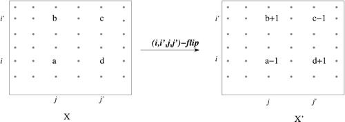
Diaconis et al. [Citation1,Citation2] define local perturbations that transform a contingency table into another of the same row and column sums. We now describe it in more detail while redefining some terms for completeness. Let be an
contingency table of row and column sums
and
, respectively. Let
be the entry on the
row and
column. That is,
is the entry in the cell
. We totally order the cells of
lexicographically. That is,
if
. If
, then
with
. A site, denoted by
, is the set of four cells
, with
and
. A flip on
is a transformation that changes the contingency table
into
by the operations
while preserving all the other entries. See for an illustration.
The following result given in [Citation1,Citation2], shows that the Markov chain on is irreducible.
Theorem 2
[Citation1,Citation2]
Given two contingency tables and
in
, there is a sequence of flips which transforms
to
.
Let denote the graph whose vertices are all
contingency tables of row and column sums
and
, respectively, and there is an edge from a vertex
to
if and only if there is a site
such that a flip on
changes
to
. If
is any vertex of
, it is routine to check that
has at most
adjacent neighbors. Indeed, the vertex
is an adjacent neighbor of
if there is a flip changing
to
. Now, given a cell
on the contingency table
, there are at most
sites involving
. Considering all
points on the array
gives a total of at most
possible sites.
For the sake of convenience, in what follows, we use or
interchangeably. We write
when we need to stress that we are talking about a contingency table and we write
if we need to stress that we are talking about the vertex that represents
in the graph
. Now, we formally define a random walk on
as follows. Start at any vertex
. If the walk is at
, choose at random an adjacent neighbor
of
, and move from
to
with probability
, or stay at
otherwise. If
denotes the transition matrix and
is the row of
corresponding to the state
, it is routine to check that the entries of
add up to 1. That is,
is a probability vector. Moreover, by Theorem 2, the matrix
is irreducible. Also, since there is a loop on every point
, the matrix
is aperiodic. Hence the random walk is an ergodic Markov chain. Finally,
is a symmetric matrix. Thus, the Markov chain has a stationary uniform distribution
. We call this Markov chain as the Diaconis Markov chain.
Theorem 3
If is the set of
contingency tables, the Diaconis Markov chain on
mixes fast and the mixing time
is given by
where
is the maximal in a cell.
We prove this result by showing that, between any two vertices of , there is a path, the canonical path, that is not ‘too long’ and where no edge is overloaded. To put this in a more formal setting, we need the following definitions and lemmas.
Let and
be two different
contingency tables. If
, we say that the point
is matched, and unmatched otherwise. Obviously therefore, to match a point
means to make
equal to
. A path from
to
is the sequence of contingency tables
, where one contingency table is obtained from the preceding one by a single flip on some site. The canonical path from
to
is a path that matches the cells in increasing lexicographic ordering. Since there are many such paths from
to
, we take the path that uses the flips with the least indices, lexicographically. This makes the canonical path unique. Suppose that at time
, the canonical path has reached the contingency table
, corresponding to matching the cell
, and
. The matched zone is the set of cells
such that
(Obviously
for
). The cell
is then called the smallest unmatched cell. A key observation, given in the lemma that follows, is that once a cell is matched, the canonical path does not unmatch it anymore. This entails that it is possible to match all the
cells in the lexicographic order, without backtracking.
Lemma 4
Let be the smallest unmatched cell at time
along the canonical path from
to
. There is a sequence of flips where all the other cells involved in matching
are greater than
.
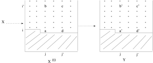
Proof
Let be the least unmatched cell at time
, and suppose that
and
, with
, as illustrated in .
If there is no row with
(if
is the last row), then
and
have different column sums on the column
, which is a contradiction. A similar argument holds if there is no column
such that
. Therefore there is a row
and column
such that
and
. Thus making
successive flips on
matches the cell
. We only have to care about the case where some entries on the site
become negative before performing all the
flips.
| 1. |
| ||||
| 2. |
| ||||
Corollary 5
For every pair of contingency tables and
, there is a sequence of flips changing
to
such that the points in successive matched zones are not affected.
Corollary 6
For all contingency tables and
, the length of the canonical path from
to
is at most
, where
is the maximal value in a cell.
Proof
To match the point requires at most
successive flips. Since there are at most
points to match and there is no backtracking by Corollary 5, the result follows.
A second key observation, given in Lemma 9, is that the number of canonical paths which pass through an edge is not too great. We first need the following definition and a lemma of far reaching importance.
Let denote the set of
contingency tables, where
and
are the sums of row
and column
, respectively, for
,
, and let
. A margin is either a column or a row sum. Let
denote the
th column of
. Suppose that the column
contains
entries and the sum of these
entries is
, then the number of non-negative integer solutions of the equation
is equal to
. We denote by
the
th non-negative integer solution of the equation
. (Not to be confused with
, the
th entry of the contingency table
.) Let
be a contingency table whose
th column is the solution
. (By Theorem 2, starting from
, it is possible to reach any
. We assume that
. We denote by
the contingency table obtained by deleting column
from
. Obviously,
is an
contingency table whose row sums are
, where
is the
th entry of column
of
. We now state and prove the following instrumental lemma.
Lemma 7
Let denote the set of
contingency tables where
and
are the sums of row
and column
, respectively, for
,
. Let
be the cardinality of
. Choose any contingency table
and let
be the column or row of
with the smallest margin amongst all the columns and rows of
. Then,
(1)
(1) where
is the number of
contingency tables that can be reached from
through a sequence of flips,
is the number of non-negative integer solutions of the equation
, and
is the margin of
.
Proof
(We insist that may be a row or a column, as long as it has the least margin. But even when it is a row, we still consider it as a column, by just transposing the table.) Consider any contingency table
and consider its column
. The set
is the disjoint union of
and
, where
is the set of contingency tables obtained from
through a sequence of flips on sites not containing entries of column
, and
is the set of contingency tables obtained from
through a sequence of flips where at least one site containing entries of column
is involved. The set
is isomorphic to the set of
contingency tables that can be reached from
after a sequence of flips. Thus,
.
Elements of the set can be obtained from
by performing a single flip in a site containing entries of column
of
to obtain a contingency table
, and, from
perform all the possible flips in sites not containing entries in column
of
. As above, this is isomorphic to the set of
contingency tables reachable from
. There are
such contingency tables. Recursively, one may thus obtain all the
, starting from
, where
, is the number of non-negative integer solutions of the equation
.
It only remains to show that each of these solutions would yield a valid contingency table in . For a contradiction, let
be a non-negative integer solution of the equation
and there is no contingency table
such that
is its
th column. Then there is no contingency table in
whose
th column can be transformed into
through a sequence of flips. Let
and
be two entries in
. We may assume that
is in the
th position (row) and
is in the
th position. There is no contingency table
in
such that
is its
th column only if there is no contingency table
in
whose
th entry is
and the
th entry is
, and such that a flip in the site
of
produces
. This is possible only if, in
, all the entries in row
(apart from
) are zeros (so that none can be decreased by 1). Thus either (1),
, where
is the sum of row
, or (2), there is another entry that is not zero in row
.
| (1) |
| ||||
| (2) | Suppose there is another entry that is not zero in row | ||||
Therefore, for all contingency tables in
whose
th entry is
and
th entry is
, and all other entries are equal to the corresponding entries of
, we have either
or
. Thus
or
. In either case,
is not a non-negative integer solution of the equation
. This is a contradiction.
Corollary 8
Let be the number of all
contingency tables of fixed row and column sums. The number of contingency tables having
fixed cells (in lexicographic ordering) is at most
.
Proof
We prove the result by induction on , the number of cells that are fixed in the lexicographical ordering. Indeed, if
, the number of such contingency tables is
. In case
, there is only a single contingency table. Hence the formula holds for these two extreme cases.
For the induction, assume that the result holds for . Let
cells be fixed and let the
cell be on the column
. Let
denote the set of contingency tables having
vertices fixed (in lexicographic ordering). We have to show that
.
By Lemma 7, and by induction, we have that
Lemma 9
If is an arc of
, then the number of different canonical paths passing through
is at most
, where
is the number of vertices of
.
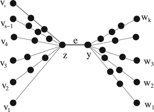
Proof
Let be a canonical path passing through the edge
, as illustrated in . In the graph
, the edge
represents a flip on a fixed site of the contingency table
, such that making the flip
moves the chain from
to
. Suppose that the
is reached at the
th flip along the canonical path
, and let
be the matched zone at
. That is,
is the set containing the first
cells, in the lexicographic ordering, i.e.,
. Now, by Lemma 4, the matched zone is preserved along the canonical path. Thus
is the end point of a canonical path passing through
only if
contains
. Hence
are contingency tables where the sequence of cells
is fixed, and the sequence of cells
may take any entry, subject to being a contingency table of the correct size. The number of such vertices (contingency tables) is thus at most
, by Lemma 7.
Moreover, let denote the complement of
. That is
. The contingency table
is the start point of the canonical path
only if
is such that matching the
first cells simultaneously turns the sequence of entries in
equal to the corresponding entries in
. Hence, since the canonical path is unique, the sequence of entries in
uniquely determines the sequence of entries in
. Therefore
are contingency tables where the sequence of cells
is uniquely determined by the sequence of cells
. The latter may take any entry, subject to being a contingency table of the right size. The number of such vertices (contingency tables) is thus at most
.
Hence, the number of canonical paths using is at most
.
Now, we are able to prove Theorem 3.
Proof of Theorem 3
In order to prove Theorem 3 by using Theorem 1, we show that there is a flow such that
is a polynomial in
, the size of contingency tables in
. Indeed, if
and
are two vertices of
, let
denote the canonical path from
to
and let
be a flow consisting of injecting
units of flow along
. Then, for all arcs
, we have
where the sum is over all the pairs
such that
. Since by Lemma 9, there are at most
canonical paths through
, and
, as the distribution
is uniform, we have
Moreover, since if there is an edge from
to
, we have
is constant for all
Thus
.
Now, using Theorem 1, Corollary 6, we have
Since an entry may take any value from to
, we have
. Thus,
Notes
Peer review under responsibility of Kalasalingam University.
References
- Diaconis P. Gangolli A. Rectangular arrays with fixed margins Proceedings of the Workshop on Markov Chains 1994 Institute of Mathematics and its Applications, University of Minnesota
- Diaconis P. Efron B. Testing for independence in a two-way table Ann. Statist. 13 1985 845 913
- Goteli N.J. Ellison A.M. A Primer of Ecological Statistics Second ed. 2013 Sinauer Associates, Inc
- Pirzada S. An Introduction To Graph Theory 2012 Universities Press OrientBlackswan, Hyderabad, India
- Brualdi R.A. Matrices of zeroes and ones with fixed row and column sum vectors Linear Algebra Appl. 33 1980 159 231
- Cobb G.W. Chen Y. An application of Markov Chains Monte Carlo to community ecology Amer. Math. Monthly 110 2003 265 288
- Cooper C. Dyer M. Greenhill C. Sampling regular graphs and Peer-to-Peer network Combin. Probab. Comput. 16 2007 557 594
- Erdös P. Gallai T.G. Graphs with prescribed degrees of vertices (Hungarian) Mat. Lapok 11 1960 264 274
- Gail M. Mantel N. Counting the number of rxc contingency tables with fixed margins J. Amer. Statist. Assoc. 72 1977 859 862
- Jerrum M. Sinclair A. Approximating the permanent SIAM J. Comput. 18 6 1989 1149 1178
- Kannan R. Tetali P. Vempala S. Simple Markov-chain algorithms for generating bipartite graphs and tournaments Random Struct. Algorithms 14 4 1999 293 308
- Sinclair A. Improved bounds for mixing rates of Markov chains and multicommodity flow Lect. Notes Comput. Sci. 583 1992 474 487
- R. Kannan, Markov Chains and polynomial time Algorithm, in: Plenary Talk At Proc. of 35th Annual IEEE Symp. on the Foundations of Computer Science, 1994, pp. 656–671.
- Erdös P.L. Miklós I. Toroczkai Z. A simple Havel-Hakimi type algorithm to realize graphical degree sequences of directed graphs Electron. J. Combin. 17 1 2010 P66
- Chen Y. Diaconis P. Holmes S. Liu J.S. Sequential Monte Carlo methods for statistical analysis of tables J. Amer. Statist. Assoc. 100 2005 109 120
- Chung F.R.K. Graham R.L. Yau S.T. On sampling with Markov chains Random Struct. Algorithms 9 1996 55 77
- Levin D.A. Peres Y. Wilmer E.L. Markov Chains and Mixing Times 2006 Amer. Math. Soc