
 ?Mathematical formulae have been encoded as MathML and are displayed in this HTML version using MathJax in order to improve their display. Uncheck the box to turn MathJax off. This feature requires Javascript. Click on a formula to zoom.
Abstract
Let be simple connected graphs on
and
vertices, respectively. Let
be a specified vertex of
and
. Then the graph
obtained by taking one copy of
and
copies of
and then attaching the
th copy of
to the vertex
,
, at the vertex
of
(identify
with the vertex
of the
th copy) is called a graph with
pockets. In 2008, Barik raised the question that ‘how far can the Laplacian spectrum of
be described by using the Laplacian spectra of
and
?’ and discussed the case when
in
. In this article, we study the problem for more general cases and describe the Laplacian spectrum. As an application, we construct new nonisomorphic Laplacian cospectral graphs from the known ones.
1 Introduction
Throughout this article we consider only simple graphs. Let be a graph with vertex set
and edge set
. The adjacency matrix of
, denoted by
, is the
matrix whose
-th entry is
, if
and
are adjacent in
and
, otherwise. The Laplacian matrix of
is defined as
, where
is the diagonal degree matrix of
It is well known that
is a symmetric positive semidefinite matrix. Throughout this paper the Laplacian spectrum of
is defined as
where
are the eigenvalues of
arranged in nondecreasing order. For any graph
and is afforded by the all ones eigenvector
There is an extensive literature on works related to Laplacian matrices and their spectra. Interested readers are referred to [Citation1,Citation2] and the references therein.
Two graphs are said to be Laplacian cospectral if they share same Laplacian spectrum. Haemers and Spence [Citation3] enumerated the numbers for which there are at least two graphs with the same Laplacian spectrum and gave some techniques for their construction.
From literature we find many operations defined on graphs such as disjoint union, complement, join, graph products (Cartesian product, direct product, strong product, lexicographic product, etc.), corona and many variants of corona (like edge corona, neighborhood corona, edge neighborhood corona, etc.). For such operations often it is possible to describe the Laplacian spectrum of the resulting graph using the Laplacian spectra of the corresponding constituting graphs, see [Citation4,Citation5] for reference. This enables one to visualize a complex network in terms of small simple recognizable graphs whose Laplacian spectra is easily computable. It is always interesting for researchers in spectral graph theory to define some new graph operations such that the Laplacian spectra of the new graphs produced can be described using the Laplacian spectra of the constituent graphs.
If and
are two graphs on disjoint sets of
and
vertices, respectively, their union is the graph
, and their join is
, the graph on
vertices obtained from
by adding new edges from each vertex of
to every vertex of
. Note that, here
denotes the complement graph of the graph
.
The following result which describes the Laplacian spectrum of join of two graphs is often used in the next sections.
Theorem 1
[Citation6], Theorem 2.1
Let be graphs on disjoint sets of
vertices respectively, and
Let
and
Then
The following graph operation is defined in [Citation7].
Definition 2
[Citation7]
Let be connected graphs,
be a specified vertex of
and
. Let
be the graph obtained by taking one copy of
and
copies of
, and then attaching the
th copy of
to the vertex
at the vertex
of
(identify
with the vertex
of the
th copy). Then the copies of the graph
that are attached to the vertices
are referred to as pockets, and
is described as a graph with pockets.
Suppose that and
are graphs on
and
vertices, respectively. Using the above operation, we can produce many interesting classes of graphs. Since the operation is a very general operation, in [Citation7], the author has asked the question that ‘how far can the Laplacian spectrum of
be described by using the Laplacian spectra of
and
?’. In that paper, the author has described the Laplacian spectrum of
using the Laplacian spectra
and
in a particular case when
. This motivates us for studying the Laplacian spectrum of more such graphs relaxing condition that
. Let
. In this case, we denote
more precisely by
. When
, we denote
simply by
.
Let . When
, we have
. Now using Theorem 1, the Laplacian spectrum of
can be obtained from that of
. So the question of describing the Laplacian spectrum of
in terms of the Laplacian spectra of
and
is same as asking for the description of the Laplacian spectrum of
in terms of the Laplacian spectra of
and
. Further, when
and
, we have
, the corona of
and
(see [Citation8]). In [Citation9], the Laplacian spectrum of
has been completely described using the Laplacian spectra of
and
.
Now if , let
, be the neighborhood set of
in
. Let
be the subgraph of
induced by the vertices in
and
be the subgraph of
induced by the vertices which are in
. When
, we describe the complete Laplacian spectrum of
using that of
and
. The results are contained in Section 2 of the article.
Further, except eigenvalues, we describe all other eigenvalues of
and prove that the remaining
eigenvalues are independent of the graphs
and
. In particular, when
, where
is the subgraph of
induced by the vertices
, we describe the complete Laplacian spectrum of
. These results are contained in Section 3.
Following notations are being used in rest of the paper. The vector with each entry
is denoted by
. The Kronecker product of matrices
is defined to be the partitioned matrix
and is denoted by
The vector with
th entry equal to
and all other entries zero is denoted by
. By
we denote the matrix of order
whose entries are all equal to
. If
, we write
simply by
. By
we denote the identity matrix of size
. We avoid writing the order of these matrices if it is clear from the context.
and
denote the complete graph and cycle graph of order
, respectively.
2 Laplacian spectrum of 
Let be a connected graph with vertex set
. Let
be a connected graph on
vertices with a specified vertex
and
. Let
. Note that
has
vertices.
Let . Without loss of generality assume that
. Let
be the subgraph of
induced by the vertices
and
be the subgraph of
induced by the vertices
. Suppose that
.
Let denote the
th vertex of
in the
th copy of
in
, for
, and let
. Then
is a partition of
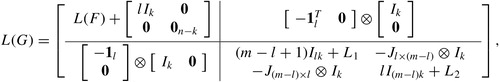
. Using this partition, the Laplacian matrix of
can be expressed as
The following is one of the main results of this article, which describes the complete Laplacian spectrum of using that of
and
.
Theorem 3
Let be a connected graph on
vertices and
be a graph on
vertices
, with a specified vertex
with degree
. Let
and
be the subgraph of
induced by the vertices
and
be the subgraph of
induced by the vertices
. Suppose that
. Let
,
and
Then the Laplacian spectrum of
consists of
| (i) | the roots of the equation | ||||
| (ii) |
| ||||
| (iii) |
| ||||
Proof
To prove part (i), suppose that are the eigenvectors of
corresponding to the eigenvalue
, respectively. Now for
, consider a vector of the form
where
and
are two arbitrary constants.
is an eigenvector of
corresponding to an eigenvalue
(say) if and only if it satisfies the equation
, which gives the following system of equations
Eliminating
and
, we get
Hence part (i) follows.
To prove part (ii) and (iii), let be the eigenvectors of
corresponding to the eigenvalues
, respectively. Similarly, let
be the eigenvectors of
corresponding to the eigenvalues
, respectively. Note that, for
and
,
and
are orthogonal to
and
, respectively. Hence for
;
;
;
are eigenvectors of
corresponding to the eigenvalues
and
, respectively. Hence the proof. □
The following example illustrates the above theorem.
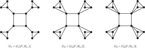
Example 4
Consider the graphs and
. Taking
and
, we have graphs
, and
, respectively. See . It can be checked that
and
, where the exponents within parenthesis indicate the multiplicities (number of occurrence) of the corresponding eigenvalues. Then the Laplacian spectrum of
are (computed through a matlab program)
One can check that matches with that obtained using the above theorem.
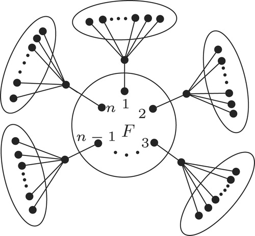
Remark 5
In a particular case, if we take and
, the empty graph on
vertices (in Theorem 3), we will get an interesting class of graphs. See . Notice that this class is nothing but the class of graphs obtained by taking a graph
on
vertices and then taking
copies of a star on
vertices and attaching one pendant vertex of
th copy of the star to the
th vertex of
. The complete Laplacian spectra of these graphs can be described easily using Theorem 3.
Remark 6
As , substituting the value in the equation given in Theorem 3 (ii), we get
whose roots are
and
. So
is always an eigenvalue of
, with corresponding eigenvector
Remark 7
In Theorem 3, . Since
and
, we have
. Thus, using Theorem 1, the Laplacian spectrum of
consists of the eigenvalues
So, notice that all the eigenvalues of
are also the eigenvalues of
. Further, except
and
, all other eigenvalues of
are of multiplicity at least
in
.
The following is auseful corollary of Theorem 3 which describes a construction of new Laplacian cospectral graphs from known pairs of nonisomorphic Laplacian cospectral graphs.
Corollary 8
Let and
are pairs of nonisomorphic Laplacian cospectral graphs on
and
vertices, respectively. Construct the graphs
and
on
vertices such that
and
. Then the graphs
and
are Laplacian cospectral, when
and
are pairwise nonisomorphic Laplacian cospectral graphs.
Proof
Proof is immediate from Theorem 3. □
Remark 9
If and
are pairs of nonisomorphic Laplacian cospectral graphs on
and
vertices, respectively, then by taking different combinations of them one can have at least
nonisomorphic Laplacian cospectral graphs which are Laplacian cospectral to
, where
.
When is not expressible as
for any
and
, we still can describe some of the Laplacian eigenvalues of
.
Theorem 10
Let be a connected graph on
vertices and
be any graph on
vertices with a specified vertex
. Then the Laplacian spectrum of
is contained in the Laplacian spectrum of
. Furthermore, if
is an eigenvalue of
afforded by an eigenvector
such that its
th component,
, then
is in the Laplacian spectrum of
occurring at least
times.
Proof
Observe that the Laplacian matrix of can be expressed as
Without loss of generality, let us assume that the vertex
be the first vertex of
. Let
be an eigenvector of
corresponding to an eigenvalue
(say) such that
. Let
. Now it can be observed that
is an eigenvector of
corresponding to the eigenvalue
.
Finally, if is an eigenvalue of
afforded by an eigenvector
such that its
th component,
, then
, for
, are the eigenvectors of
corresponding to the eigenvalue
, where
. Hence the result. □
3 Laplacian spectrum of a graph with pockets
In this section, we consider the case when is not necessarily equal to
. Let
be a connected graph with vertex set
. Let
be a graph on
vertices with a specified vertex
and
. Let
. Without loss of generality, assume that
. Let
be the subgraph of
induced by the vertices
and
be the subgraph of
induced by the vertices
. Suppose that
.
Let be the graph obtained by taking one copy of
and
copies of
, and then attaching the
th copy of
to the vertex
at the vertex
of
(identify
with the vertex
of the
th copy). In general, it is difficult to characterize all the Laplacian eigenvalues of
. In the following theorem we describe
eigenvalues of
and prove that the remaining
eigenvalues are independent of thegraph
.
Theorem 11
Let be the graph as described above. Suppose that
,
. Let
, where
. Then
for
and
for
are eigenvalues of
each of multiplicity
, and the other
eigenvalues are independent of the graph
. That is, if
| (i) |
| ||||
| (ii) |
| ||||
| (iii) |
| ||||
then
| (i) |
| ||||
| (ii) |
| ||||
| (iii) |
| ||||
Proof
The Laplacian matrix of can be expressed as
where
and
. So the Laplacian matrix of
can be related to
as
Now, suppose that
are the eigenvectors of
corresponding to the eigenvalues
, respectively. Similarly, let
be the eigenvectors of
corresponding to the eigenvalues
, respectively. Then observe that for
;
;
,
are eigenvectors of
corresponding to the eigenvalues
and
, respectively. Similarly, for
;
;
,
are eigenvectors of
corresponding to the eigenvalues
and
, respectively. Furthermore, by choosing vectors of the form
for some
, we get the same set of eigen-equations for
and
. Hence the result follows. □
Now, consider the case when , where
is the subgraph of
induced by the vertices
and
is the subgraph of
induced by the vertices
. In this case, we describe the Laplacian matrix and the complete Laplacian spectrum of
.
Let denote the
th vertex of
in the
th copy of
in
, for
, and let
. Then
is a partition of the vertex set of
. Using this partition, the Laplacian matrix of
can be expressed as
where
, and
The following result describes the complete Laplacian spectrum of .
Theorem 12
Let be the graph as described above. Let
,
,
, and
. Then the Laplacian spectrum of
consists of the eigenvalues as
| (i) |
| ||||
| (ii) | the roots of the equation | ||||
| (iii) | for | ||||
| (iv) |
| ||||
| (v) |
| ||||
Proof
Proof of part (i) is trivial.
To prove part (ii), consider the vector where
and
are some arbitrary constants. Then
would be an eigenvector for
if it satisfies the matrix equation
for some
, which after simplification gives the following system of equations
in
unknowns
and
. Now eliminating
and
, we get
Hence we get result (ii).
To prove (iii), suppose that are the eigenvectors of
corresponding to the eigenvalues
, respectively. Now for
, consider the vectors
where
and
are two arbitrary constants. From the eigen-equations, we have
Then solving the above equations for
, we have the required result.
To prove (iv), suppose that are eigenvectors of
corresponding to the eigenvalues
, respectively. Consider the vectors
for
. Now using Theorem 1, it can be observed that
is an eigenvector of
corresponding to the eigenvalue
, for
. Hence the proof.
Proof of part (v) follows directly from parts (ii) and (iii) of Theorem 3. □
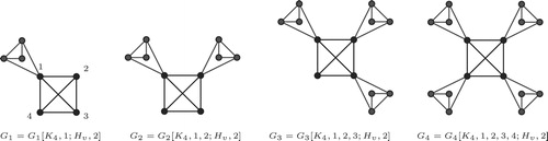
Example 13
Consider the four graphs and
shown in , obtained from the two graphs
and
such that
. Observe that,
has one pocket and in this case
and
. Similarly,
,
and
are graphs with
,
, and
pockets, respectively.
It can be checked that and
and
Notice that
matches with that obtained as described in the above theorem.
Remark 14
Let Now (iii) and (iv) of Theorem 12 can be stated in terms of
as follows. If
, then all the roots of
belong to
. Furthermore, if
, then
.
The following corollary gives a construction of new Laplacian cospectral graphs from the known ones.
Corollary 15
Let and
be pairs of nonisomorphic Laplacian cospectral graphs on
and
vertices, respectively. Let
,
,
and
. Let
and
. Then the graphs
and
(each with
pockets) are Laplacian cospectral.
Proof
Proof follows from Theorem 12. □
Notes
Peer review under responsibility of Kalasalingam University.
References
- Bapat R.B. Graphs and Matrices 2011 Springer
- Merris R. Laplacian matrices of graphs: a survey Linear Algebra Appl. 197 1994 143 176
- Haemers W.H. Spence E. Enumeration of cospectral graphs European J. Combin. 25 2004 199 211
- Brouwer A.E. Haemers W.H. Spectra of Graphs 2011 Springer Science & Business Media
- Cvetković D.M. Doob M. Sachs H. Spectra of Graphs-Theory and Applications 1979 Academic Press New York
- Merris R. Laplacian graph eigenvectors Linear Algebra Appl. 278 1998 221 236
- Barik S. On the Laplacian spectra of graphs with pockets Linear Multilinear Algebra 56 2008 481 490
- Harary F. Graph Theory 1969 Addison-Wesley Reading, MA
- Barik S. Pati S. Sarma B.K. The spectrum of the corona of two graphs SIAM J. Discrete Math. 24 2007 47 56