
 ?Mathematical formulae have been encoded as MathML and are displayed in this HTML version using MathJax in order to improve their display. Uncheck the box to turn MathJax off. This feature requires Javascript. Click on a formula to zoom.
Abstract
Rosa, in his classical paper (Rosa, 1967) introduced a hierarchical series of labelings called and
labeling as a tool to settle Ringel’s Conjecture which states that if
is any tree with
edges then the complete graph
can be decomposed into
copies of
. Inspired by the result of Rosa, many researchers significantly contributed to the theory of graph decomposition using graph labeling. In this direction, in 2004, Blinco, El-Zanati and Vanden Eynden introduced
-labeling as a stronger version of
-labeling. A function
defined on the vertex set of a graph
with
edges is called a
-labeling if
(i) is a
-labeling of
,
(ii) is tripartite with vertex tripartition
with
and
such that
is the unique edge joining an element of
to
,
(iii) for every edge with
,
,
(iv) .
Further, Blinco et al. proved a significant result that if a graph with
edges admits a
-labeling, then the complete graph
can be cyclically decomposed into
copies of the graph
, where
is any positive integer. Motivated by the result of Blinco et al., we show that a new family of almost bipartite graphs each admits
-labeling. The new family of almost bipartite graphs is defined based on the supersubdivision graph of certain connected graph. Supersubdivision graph of a graph was introduced by Sethuraman and Selvaraju in Sethuraman and Selvaraju (2001). A graph is said to be a supersubdivision graph of a graph
with
edges, denoted
if
is obtained from
by replacing every edge
of
by a complete bipartite graph
,
, (where
may vary for each edge
) in such a way that the ends of
are identified with the 2 vertices of the vertex part having two vertices of the complete bipartite graph of
after removing the edge
of
. In the graph
, the vertices which originally belong to the graph
are called the base vertices of
and all the other vertices of
are called the non-base vertices of
. More precisely, we prove that if
is a connected graph containing a cycle
, where
and having a vertex of degree two with one of its adjacent vertices of degree one and its other adjacent vertex is of degree at least two, then certain supersubdivision graph of the graph
,
plus an edge
admits
-labeling, where
is added between a suitably chosen pair of non-base vertices of the graph
. Also, we discuss a related open problem.
1 Introduction
Decomposition of a graph is a system
of subgraphs of
such that any edge of the graph
belongs to exactly one of the subgraphs in
. A decomposition
of a graph
is said to be cyclic if
contains a graph
then it also contains the graph
obtained by turning
. In an attempt to settle the Ringel’s Conjecture that if
is any tree with
edges then the complete graph
can be decomposed into
copies of
, Rosa in his classical paper [Citation1] introduced a series of labelings called
and
labeling.
A one-to-one function from the vertex set of a graph
with
edges to the set
is called a
-labeling of
if
. Let
be a graph with
edges. A one-to-one function
is called a
-labeling of
if
.
-labeling of a graph
with
edges is a one-to-one function
such that
.
-labeling was later called as graceful labeling by Golomb [Citation2] and this term is most widely used. A
-labeling
of a graph
with
edges is called an
-labeling if there exists an integer
such that
or
for every edge
. It is clear that
-labeling is a stronger version of
-labeling,
-labeling is a weaker version of
-labeling and
-labeling is a stronger version of
-labeling.
Further, Rosa [Citation1] proved the following two significant theorems.
Theorem 1.1
If is a graph with
edges, then there exists a cyclic
-decomposition of
if and only if
has a
-labeling.
Theorem 1.2
Let be a graph with
edges that has an
-labeling. Then there exists a cyclic
-decomposition of
into subgraphs isomorphic to
, where
is an arbitrary natural number.
The above two results inspired many researchers to discover similar labelings that can be used as a tool for decomposition of complete graphs or complete multipartite graphs. In this direction in [Citation3] El-Zanati et al. introduced -labeling. Let
be bipartite graph with
edges and bipartition
.
-labeling of
is a one-to-one function
such that the integers
are distinct modulo
over all ordered pairs
with
and
whenever
,
and
. They have also proved the following decomposition theorem.
Theorem 1.3
If a bipartite graph with
edges has a
-labeling and
is any positive integer then there exists a cyclic
-decomposition of
.
In [Citation4] Fronček introduced blended -labeling. Let
be a graph with
edges,
,
and
. Let
be an injection,
,
. The pure length of an edge
with
,
is defined as
for
and the mixed length of an edge
is defined as
mod
for
.
has a blended
-labeling if
| (i) |
| ||||
| (ii) |
| ||||
Using the blended -labeling Fronček [Citation4] proved the following decomposition theorem.
Theorem 1.4
Let the graph with
edges have a blended
-labeling. Then there exists a bi-cyclic decomposition of
into
copies of
.
In [Citation5] Fronček and Kubesa have examined about the decomposition of the complete graph into
isomorphic spanning trees using a new type of labeling called switching blended labeling. For more details refer [Citation5]. In 2013, Anita Pasotti [Citation6] introduced a generalization of graceful labeling called
-divisible graceful labeling as a tool to obtain cyclic
-decomposition in complete
-partite graphs with parts of size
,
. Let
be a graph of size
and let
be a divisor of
, say
. A
-divisible graceful labeling of
is an injective function
such that
. A
-divisible
-labeling of a bipartite graph
is a
-divisible graceful labeling of
having the property that its maximum value on one of the two bipartite sets does not reach its minimum value on the other one.
Further, Anita Pasotti [Citation6] has proved the following significant theorems.
Theorem 1.5
If there exists a -divisible graceful labeling of a graph
of size
then there exists a cyclic
-decomposition of
.
Theorem 1.6
If there exists a -divisible
-labeling of a graph
of size
then there exists a cyclic
-decomposition of
for any positive integer
.
With the motivation to decompose the complete graph into almost-bipartite graphs with
edges, where
is any positive integer, Blinco et al. [Citation7] introduced
-labeling (A graph is said to be almost-bipartite if the removal of a particular edge makes the graph bipartite). A function
defined on the vertex set of a graph
with
edges is called a
-labeling if
| (i) |
| ||||
| (ii) |
| ||||
| (iii) | for every edge | ||||
| (iv) |
| ||||
Further, in [Citation7], Blinco et al. have proved the following significant theorem.
Theorem 1.7
Let be a graph with
edges having
-labeling. Then there exists a cyclic
-decomposition of
, where
is any positive integer.
Inspired by the above result of Blinco et al., the almost-bipartite graphs ,
,
,
,
,
,
,
,
,
,
,
,
,
are found to have
-labeling (refer [Citation8–10,7,11]). For survey on
-labeling refer the survey on graph labeling by Gallian [Citation12]. In [Citation13], Sethuraman and Selvaraju introduced a graph operation called supersubdivision of a graph that generate families of bipartite graphs from the given graph. Let
be a graph with
edges. A graph is said to be a supersubdivision graph of a graph
with
edges, denoted
if
is obtained from
by replacing every edge
of
by a complete bipartite graph
,
, (where
may vary for every edge
) in such a way that the ends of
are identified with the 2-vertex part of
after removing the edge
from
. (In the complete bipartite graph
the part consisting of two vertices is referred as 2-vertex part of
and the part consisting of
vertices is referred as
-vertex part of
). Note that for
, if
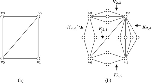
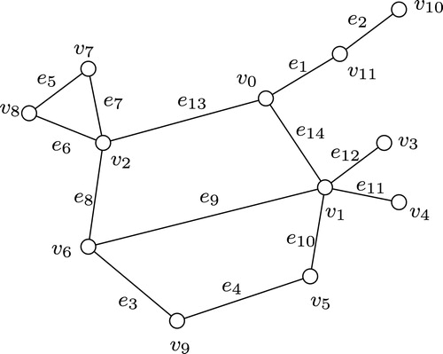
for any particular edge in the supersubdivision then this results in the classic definition of subdividing a single edge. Supersubdivision graph of the graph in (a) is shown in (b).
Fig. 1 (a) The graph (b) Supersubdivision graph of the graph
.
In [Citation14] we have proved that a family of almost bipartite graphs obtained from the supersubdivision of any tree with at least three vertices admits -labeling and we posed an open problem that whether supersubdivision of any connected graph plus an edge admits
-labeling. We partially answer this question by proving the following result. Let
be a connected graph containing a cycle
, where
and having a vertex of degree two with one of its adjacent vertices of degree one and its other adjacent vertex is of degree at least two. Then certain supersubdivision graph of the graph
,
plus an edge
admits
-labeling, where
is added between a suitably chosen pair of non-base vertices of the graph
. Also, we discuss a related open problem.
2 Main result
In this section we first present Algorithm 1 to construct supersubdivision graph of a connected graph containing a cycle , where
and having a vertex of degree two with one of its adjacent vertices of degree one and its other adjacent vertex is of degree at least two. Then we prove that certain supersubdivision graph of the graph
,
plus an edge
admits
-labeling, where
is added between a suitably chosen pair of non-base vertices of the graph
.
Algorithm 1
Construction of Supersubdivision Graphs Input. Any connected graph containing a cycle
, where
and having a vertex of degree two with one of its adjacent vertices of degree one and its other adjacent vertex is of degree at least two.
Step 1. Naming the vertices of by BFS algorithm.
Find a vertex of degree two having one adjacent vertex with degree one and the other adjacent vertex with degree at least two. Refer such a vertex of degree two by , its unique adjacent vertex of degree one by
and the unique adjacent vertex of degree at least two by
. Obtain the graph
, denote the graph thus obtained as
. Considering the vertex
as the root of
, run BFS on
and obtain the BFS ordering of the vertices in
as
, where
is the root
and
. Then name the vertex
as
and
as
in the graph
. [Thus, the vertices of
are ordered (or named) as
].
Step 3. Edge ordering
Denote the edges as
respectively. Among all the adjacent vertices of
, find the vertex with label having the largest index, say
. Then denote the edge
by
. Then find the adjacent vertex of
with the label having the largest possible index less than
, say
. Then denote the edge
by
. Similarly, sequentially find the adjacent vertices
of
and label the edges
by
, where
is the degree of
and
. For
,
in the increasing order of
, find the adjacent vertices of
, then label the incident edges at
in the increasing order of
sequentially as done above as
, where
denotes the number of edges of the graph
.
Step 4. Defining basic labels
Define , for
,
.
Step 5. Edge replacement
Step 5.1. Replacement of the edge
Replace the edge by
, where
is any positive integer in such a way that the ends
and
of
are identified with the 2-vertex part of
.
Step 5.2. Replacement of the edge
Replace the edge by
in such a way that the ends
and
of
are identified with the 2-vertex part of
, where
is defined depending on the congruence class of
modulo 4 as given in .
Table 1 Value of depending on the congruence class of
modulo 4.
Step 5.3. Replacement of the edge .
Replace the edge by
in such a way that the ends
and
of
are identified with the 2-vertex part of
, where
is defined depending on the nature of
as given in .
Table 2 Value of depending on the nature of
.
Step 5.4. Replacement of the edge for
,
.
Replace every edge for
,
by
, where
,
,
is an arbitrary positive integer in such a way that the end vertices of
are identified with the 2-vertex part of
.
Notation 1
For a given connected graph , the supersubdivision graph of
constructed by Algorithm 1 is denoted by
.
Notation 2
The vertex set of the graph ,
can be partitioned into two sets
and
, where
is the set of all actual vertices of
in
called base vertices of
and
is the set of vertices which lie in the
-part of the complete bipartite graph
which replaces the edge
of
in construction of the graph
, for
and they are called non-base vertices of
.
Theorem 2.1
Let be a connected graph containing a cycle
, where
and having a vertex of degree two with one of its adjacent vertices of degree one and its other adjacent vertex is of degree at least two. Then certain supersubdivision graph of the graph
,
plus an edge
admits
-labeling, where
is added between a suitably chosen pair of non-base vertices of the graph
.
Proof
Let be a connected graph containing a cycle
, where
and having a vertex of degree two with one of its adjacent vertices of degree one and its other adjacent vertex is of degree at least two. Then, the supersubdivision graph of the graph
,
is obtained by using Algorithm 1. Consider the graph
, where
is the new edge joining any two of the non-base vertices say
and
of the
-vertex part of the complete bipartite graph
which replaces the edge
of the graph
. From the construction, we observe that, the graph
has
vertices and
edges, where
is the number of vertices of the graph
,
is the number of edges of the graph
and
is the number of vertices in the
-part of
which replaces the edge
in constructing
, for
. That is,
and
.
By Notation 2, , where
is the set of base vertices of
and
is the set of non-base vertices of
.
Defining vertex labeling on the base vertices of
.
Define , for
,
.
Defining vertex labeling on the non-base vertices of
.
First we define labels on the non-base vertices of the complete bipartite graphs ,
which replace the edges
,
respectively in constructing
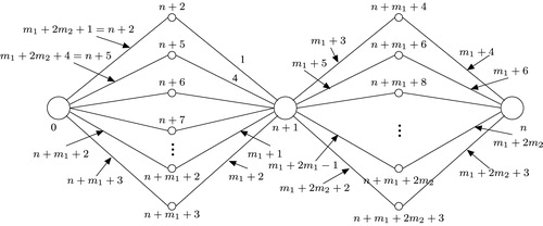
, as shown in .
Fig. 2 Labels of vertices and edges of and
.
For , we find all the adjacent vertices
of
satisfying the index property
. [Note that, here
denotes the number of such adjacent vertices of
] For each
,
and for
,
, we consider the edge
of
and the complete bipartite graph
which replaces the edge
in constructing
, where
is any positive integer and
is obtained as
. Now, in order to define the labels for the non-base vertices of
we introduce the following parameters.
For the case , define
, where
is defined depending on the congruence class of
modulo 4 as given in .
Table 3 Value of depending on the congruence class of
modulo 4.
Define , for
.
For each ,
, define
Then, for
and for
,
, the labels of the non-base vertices of the complete bipartite graph
which replaces the edge
of
in constructing the graph
is defined as shown in . From the above labeling given in , it is clear that, except the non-base vertices of the complete bipartite graph
which replaces the edge
, all the other non-base vertices of the complete bipartite graph
which replaces the edge
for each
,
and for
,
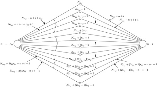
are labeled.
Fig. 3 Labels of vertices and edges of for each
,
and for
,
.
Now, we consider the complete bipartite graph which replaces the edge
in constructing
and we define labels for the non-base vertices of
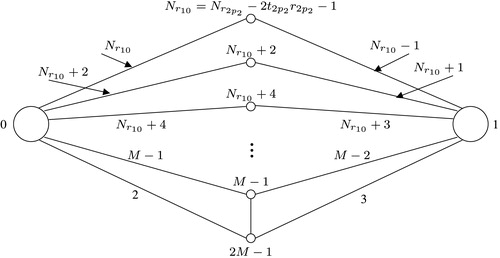
as shown in .
Fig. 4 Labels of vertices and edges of the complete bipartite graph which replaces the edge .
Observation 1
Vertex labels of are distinct.
The labels of base vertices of form an increasing sequence
. Thus they are distinct. From , it is clear that the labels of the non-base vertices of the complete bipartite graphs
and
form an increasing sequence,
Note that, maximum of
minimum of
. Thus,
is also an increasing sequence.
From the definition of , it is clear that the difference between the label of the first non-base vertex of the complete bipartite graph
which replaces the edge
and the last non-base vertex of the complete bipartite graph
which replaces the edge
is
, where the value of
is defined in .
For , from the definition of
, it is clear that the difference between the label of the first non-base vertex of the complete bipartite graph
and the label of the last non-base vertex of the complete bipartite graph
is
.
For each ,
and for
,
, from the definition of
, it is also clear that the difference between the label of the first non-base vertex of the complete bipartite graph
and the last non-base vertex of the complete bipartite graph
is
.
From , we observe that the labels of the non-base vertices in the first set of increase consecutively by one. Hence the labels of all the non-base vertices of the first set of
are distinct. Further, we observe that the least value of the labels of the first set of
is
and the largest value of the labels of the non-base vertices of the second set of
is
and their difference is
. As in the first set, the labels of the non-base vertices of the second set also increase by one consecutively. Hence, the labels of all the non-base vertices of the second set of
are also distinct. Similarly, the labels of the non-base vertices of the other remaining
sets of
are distinct.
From , observe that the labels of the non-base vertices of the complete bipartite graph form an increasing sequence,
Thus, the labels of vertices of
can be arranged as a monotonically increasing sequence. Hence the vertex labels of the graph
are distinct.
Observation 2
Edge labels of are distinct.
Since the labels of the edges are
respectively (which are beyond
), we consider their edge labels as
and
respectively. From , we observe that the labels of the edges of
and
can be arranged as the following sequences,
From , we observe that the
edges of the first set of
get distinct values from
the
edges of the second set of
get distinct values from
and finally, the
edges of the
set of
get distinct values from
Thus, the
edges of
can be arranged as a sequence,
From , the labels of the edges of
can be arranged as three sequences,
Thus, from , it is clear that the labels of edges of
can be arranged as a monotonically increasing sequence from 1 to
.
Hence the edge labels of are distinct.
Observation 3
is a
-labeling.
In order to prove that is a
-labeling, we partition the vertex set
as
, where
,
and
. Then, by the above labeling, we have
for any
and for any
.
The label of the edge .
Hence, from Observations 1–3, the graph admits
-labeling. □
Illustration
We illustrate below the -labeling that is defined as in the proof of Theorem 2.1. The connected graph
with edge labels is given in .
Fig. 5 The connected graph with edge labels.
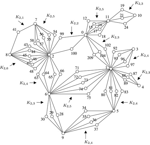
The -labeled
, where the
-labeling as defined in the proof of Theorem 2.1 is given in . Note that
.
Fig. 6 -labeling of
.
As the graph admits
-labeling, from Theorems 1.7 and 2.1 we have the following corollary.
Corollary 2.2
The complete graph can be cyclically decomposed into copies of the graph
, where
is a connected graph containing a cycle
, where
and having a vertex of degree two with one of its adjacent vertices of degree one and its other adjacent vertex is of degree at least two,
is certain supersubdivision graph of the graph
plus an edge
added between suitably chosen pair of non-base vertices of the graph
,
is any positive integer and
.
3 Discussion
In Section 2, we consider the connected graph containing a cycle
, where
and having a vertex of degree two with one of its adjacent vertices of degree one and its other adjacent vertex is of degree at least two. Then the graph
is obtained from certain supersubdivision graph of the graph
and adding an edge
between suitably chosen pair of non-base vertices in
. In Theorem 2.1 for such special connected graph
, we have shown that
admits
-labeling. We strongly feel that supersubdivision of any connected graph
with one additional edge would also admit
-labeling and also from the inspiration of the result of Sethuraman and Selvaraju [Citation15] we pose the following conjecture,
Supersubdivision of any connected graph plus an edge
,
admits
-labeling, where
is added between suitably chosen pair of non-base vertices of
.
References
- RosaA., On certain valuations of the vertices of a graph Theory of Graphs Rome, 1966 International Symposium1967Gordon and Breach, NY, Dunod Paris349–355
- GolombS.W., How to number a graphReadR.C.Graph Theory and computing1972Academic PressNew York23–37
- El-ZanatiS.I.Vanden EyndenC.PuninN., On the cyclic decomposition of complete graphs into bipartite graphs Australas. J. Combin. 242001 209–219
- FrončekD., Bi-cyclic decompositions of complete graphs into spanning trees Discrete Math. 3072007 1317–1322
- FrončekD.KubesaM., Factorizations of complete graphs into spanning trees Congr. Numer. 1542002 125–134
- PasottiA., On d-graceful labelings Ars Combin. 1112013 207–223
- BlincoA.El-ZanatiS.I.Vanden EyndenC., On the cyclic decomposition of complete graphs into almost-bipartite graphs Discrete Math. 2842004 71–81
- BlairG.W.BowmanD.L.El-ZanatiS.I.HaldS.M.PribanM.K.SebestaK.A., On cyclic C2m+e-designs Ars Combin. 932009 289–304
- BungeR.C.El-ZanatiS.I.O’HanlonW.Vanden EyndenC., On γ-labeling of the almost-bipartite graph Pm+e Ars Combin. 1072012 65–80
- El-ZanatiS.I.O’HanlonW.A.SpicerE.R., On γ-labeling of the almost-bipartite graph Km,n+e East-West J. Math. 10 2 2008 133–139
- El-ZanatiS.I.Vanden EyndenC., On Rosa-type labelings and cyclic graph decompositions Math. Slovaca 59 1 2009 1–18
- GallianJ.A., A dynamic survey of graph labeling Electron. J. Combin. 202017 #DS6
- SethuramanG.SelvarajuP., Gracefuness of arbitrary supersubdivisions of graphs Indian J. Pure Appl. Math. 32 7 2001 1059–1064
- G. Sethuraman, M. Sujasree, Generating γ-labeled graphs from any tree with at least three vertices, Indian J. Pure Appl. Math. (submitted for publication).
- SethuramanG.SelvarajuP., Decompositions of complete graphs and complete bipartite graphs into isomorphic supersubdivision graphs Discrete Math. 2602003 137–149