
 ?Mathematical formulae have been encoded as MathML and are displayed in this HTML version using MathJax in order to improve their display. Uncheck the box to turn MathJax off. This feature requires Javascript. Click on a formula to zoom.
Abstract
Acharya (1982) proved that every connected graph can be embedded in a graceful graph. The generalization of this result that, any set of graphs can be packed into a graceful graph was proved by Sethuraman and Elumalai (2005). Recently, Sethuraman et al. (2016) have shown that, every tree can be embedded in an graceful tree. Inspired by these fundamental structural properties of graceful graphs, in this paper, we prove that any acyclic graph can be embedded in an unicyclic graceful graph. This result is proved algorithmically by constructing graceful unicyclic graphs from a given acyclic graph. Our result strongly supports the Truszczynski’s Conjecture that “All unicyclic graphs except the cycle with
or 2(mod 4) are graceful”.
1 Introduction
All the graphs considered in this paper are finite and simple graphs. The terms which are not defined here can be referred from Citation[1]. In 1963, Ringel posed his celebrated conjecture, popularly called Ringel Conjecture Citation[2], which states that, , the complete graph on
vertices can be decomposed into
isomorphic copies of a given tree with
edges. Kotzig Citation[3] independently conjectured the specialized version of the Ringel Conjecture that the complete graph
can be cyclically decomposed into
copies of a given tree with
edges. In an attempt to solve both the conjectures of Ringel and Kotzig, in 1967, Rosa, in his classical paper Citation[4] introduced an hierarchical series of labelings called
and
labelings as a tool to settle both the conjectures of Ringel and Kotzig. Later, Golomb Citation[5] called
-labeling as graceful labeling, and now this term is being widely used. A function
is called graceful labeling of a graph
with
edges, if
is an injective function from
to
such that, when every edge
is assigned the edge label
, then the resulting edge labels are distinct. A graph which admits graceful labeling is called graceful graph. Further, Rosa Citation[4] proved that “If a graph
with
edges has a graceful labeling then the complete graph
can be cyclically decomposed into
copies of the graph
”. This result subsequently induced the popular Graceful Tree Conjecture, which states that “Every tree is graceful”. The Graceful Tree Conjecture appears to be hard and it remains open over 5 decades.
Rosa Citation[4] also proved that the cycle is graceful if and only if
or
(mod 4). In 1984, Truszczynski’s Citation[6] conjectured that, “All unicyclic graphs except the cycle
with
or
(mod 4) are graceful”. The conjecture of Truszczynski is also hard as the Graceful Tree Conjecture. Not much results have been proved to support Truszczynski’s Conjecture. Some of the interesting results supporting Truszczynski’s Conjecture are listed below.
| • | Barientos Citation[7] proved that a unicyclic graph in which the deletion of any edge on the cycle results in a caterpillar is graceful. [A tree is called a caterpillar, in which the removal of all the pendant vertices of the tree results in a path]. | ||||
| • | Jaya Bagga and Arumugam Citation[8] have constructed a graceful unicyclic graph from a special class of caterpillars. | ||||
| • | Figueroa-Centeno et al. Citation[9] have provided an interesting construction to form a graceful unicyclic graph from a set of | ||||
For more details on the results supporting Truszczynski’s Conjecture refer the dynamic survey on graph labeling by Gallian [Citation10]. Structural characterization of graceful graphs appears to be one of the most difficult problems in graph theory. However, some interesting general structural properties of graceful graphs are established. Acharya [Citation11] proved that every connected graph can be embedded in a graceful graph. In [Citation12], Sethuraman and Elumalai generalized this result and they have shown that every set of graphs can be packed into a graceful graph. Recently, in [Citation13] Sethuraman et al. have also shown that every tree can be embedded in a graceful tree. Inspired by these fundamental structural properties of graceful graphs, in this paper, we prove that any acyclic graph can be embedded in a graceful unicyclic graph. This result is proved algorithmically by constructing graceful unicyclic graphs from a given acyclic graph. More precisely, we prove a general result that from any given acyclic graph containing
arbitrary trees, we construct graceful unicyclic graphs with cycle length that vary from
to
. Our result strongly supports the Truszczynski’s Conjecture.
2 Main result
In this section, we present our Embedding Algorithm, which generate graceful unicyclic graphs from any acyclic graph.
Note
For convenience hereafter a vertex in either or
or
or
is referred by its label. Similarly an edge in either
or
or
or
is referred by its label. We make the following observations and prove the following lemmas to establish that the Embedding Algorithm indeed construct graceful unicyclic graphs from the input forest as the output.
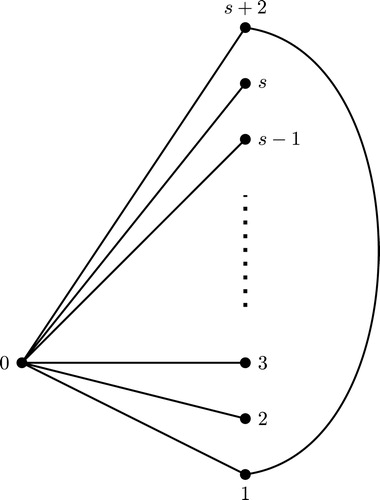
Observation 2.1
From Step 5 of the Embedding Algorithm, the vertices which appear on the left side part of the bipartition of the tree receive consecutive vertex labels from
to
and the vertices which appear on the right side of the bipartition of the tree
receive the vertex labels of the form
,
.
Observation 2.2
From Step 2 and Step 5 of the Embedding Algorithm, observe that, in the bipartite graph, all the children of the vertex
,
are arranged consecutively from top to bottom based on decreasing order of their degrees in the right side just below the last child of the vertex
. Similarly, observe that, all the children of the vertex
,
are arranged consecutively from top to bottom on the left side based on decreasing order of their degrees just below the last child of the vertex
.
Observation 2.3
From Observation 2.1, the Missing Vertex Label Set defined in Step 6.1 consists of all the labels (integers) that lie in the interval
, for all
. More precisely, the Missing Vertex Label Set
. If we arrange the elements of
as a sequence
, then any two consecutive terms,
and
, for
either both lie on the same interval say
for some fixed
or
and
for some fixed
. Thus, either
or
.
Observation 2.4
From Observation 2.1, the labels of the edges that are incident at the vertex,
must lie on the interval
. Therefore, the maximum of the edge labels of all the edges that are incident at the vertex
is less than the minimum of the edge labels of all the edges that are incident at the vertex
, for every
. The missing edge labels at the vertex
, for each
,
, is the set of labels (integers) that lie on
excluding the labels of the edges that are incident at the vertex
and it is denoted by
. More precisely the set
}. Then we can describe the set
. As
is a tree,
.
Lemma 2.5
The vertex labels as well as the edge labels of the tree obtained in Step 5 of the Embedding Algorithm are all distinct.
Proof
It follows from Observation 2.1, the labels of all the vertices of the tree are distinct.
Claim
The labels of all the edges of the tree are distinct
Since the labels of the vertices that lie on the left side part of the bipartition of are consecutive from
to
, it follows that, the labels of the incident edges at each vertex
,
are all distinct and these labels lie in the set
. Further, for any two consecutive vertices on the right side part of the bipartition of
, say
and
, we have maximum over the labels of all the edges that are incident at the vertex
minimum over the labels of all the edges that are incident at the vertex
, for
. Thus, the labels of the edges that are incident at any two distinct vertices on the right side part of the bipartition of
are always distinct. This would imply that the labels of all the edges of the tree
are distinct. □
Lemma 2.6
The sets and
, defined in Step 6.1 of the Embedding Algorithm are empty if and only if the tree
is a star.
Proof
Assume that the tree is a star with
vertices. Without loss of generality, we assume that
, where
is the bipartition of the tree
. By Step 3 of the Embedding Algorithm,
and
. After the execution of Step 5 of the Embedding Algorithm, Existing Vertex Label Set
and the Existing Edge Label Set
. As the set
, the set
and the set
.
Conversely, assume that each of the sets and
, defined in the Step 6.1 of Embedding Algorithm is empty. We claim that the tree
is a star. Suppose that the tree
is not a star. Then,
. By using Step 5 of the Embedding Algorithm, the Existing Vertex Label Set
. Since
,
. A contradiction to our assumption that
. Hence the input tree
must be a star. □
Lemma 2.7
The label defined in Step 6.3 of the Embedding Algorithm is a non-negative integer for all values of
and the label
exists as the vertex label of a vertex of the current tree
that is being used in the current execution of Step 6.3.
Proof
Observe that Step 6.3 of the Embedding Algorithm is executed when the sets and
are non-empty. Hence by Lemma 2.6, the tree
is not a star. Thus,
. Further, for every
,
,
,
, the label
is found in Step 6.3.
Claim
is a non-negative integer
To ascertain the claim we prove that , for every
,
by using induction on
.
When , from Observation 2.3, we have
and from Observation 2.4,
. Hence
.
We assume that the result is true for up to . That is, we assume that
, for each
.
We now prove that the statement is true for . More precisely, we prove that
. Suppose that
. From Observation 2.3,
and
differ either by
or
. It follows from our assumption (
) and the inductive assumption (
), that
(1)
(1) Since, either
or
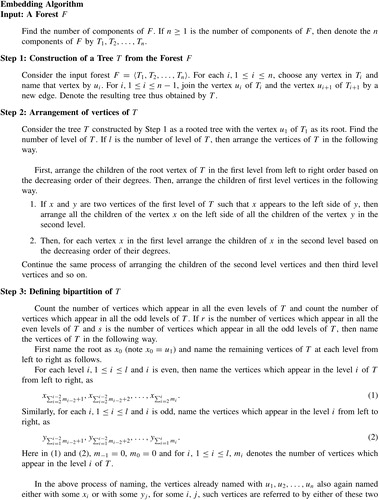
, we consider the following two cases.
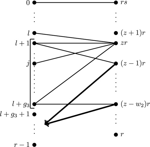
Case 1.
Since and
are consecutive missing edge labels and from Eq. (1), the labels of the sequence
are consecutive existing edges labels that lie between
and
. For whatever may be the value of
, the sequence
always contains the labels
and
. Since
and
are consecutive missing vertex labels, the label
must be an existing vertex label which appears on the right side of the bipartition of the tree
. From Step 5 of the Embedding Algorithm,
, for some
. As
belongs to
, the label
is also an existing edge label, the label
appears as existing vertex label as well as existing edge label. As
, for some
, by Observation 2.4 the edge label
is only obtained from the edge connecting the vertex
and the vertex
. The label
is the maximum edge label obtained at the vertex
. As
also belongs to
,
is the next existing edge label just after
. As by Observation 2.4, the edge label
must be obtained at the edge connecting the vertex
and the vertex
, for
. Since
is the bottommost vertex of the left side part of the bipartition of
and
is also a child of the vertex
, this would imply from our construction of the tree
, the vertex
, for each
are pendant. Hence the only vertex adjacent with
is 0. From Observation 2.4, the set
. Therefore the label
is a missing edge label. Then from Eq. (1) that,
, we have
. (See .)
Fig. 1 The structure of the bipartite tree under the Case 1.
As . By Observation 2.4,
. Since the vertex
is pendant, for each
,
,
. Thus,
. Since
and by Observation 2.3,
, we have
. But from the above discussion
. This leads to a contradiction. Therefore, our assumption that
is wrong. Hence
.
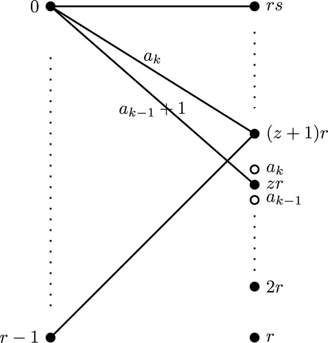
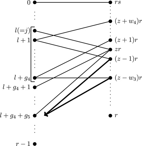
Case 2.
By Observation 2.3, the labels and
lie in the interval
, for some fixed
. Therefore,
for some
. Since
and
are consecutive missing edge labels and from Eq. (1), the labels of the sequence
are consecutive existing edges labels that lie between the label
and the label
. For whatever may be the value of
the sequence
should contain the label
. Hence, by Observation 2.4, the existing edge label
must be obtained at the edge incident with the vertices
and
, for some
.
Claim
The edge label obtained at the edge
for some
Suppose that the edge label is not obtained at the edge
, for any
. Then by Observation 2.4,
is obtained at the edge incident at the vertex
, for some
. Since the labels
are consecutive existing edge labels and the edge label
is obtained at the edge
, for some
, by Observation 2.4, the vertex
must be adjacent with the vertices
also the vertices
must all be adjacent with all the vertices on the left side part of the tree
. As
, for
, are all adjacent with the vertices
, there exists a cycle in
if
. Hence
. Suppose
, then the vertex
must be adjacent with the vertices
,
[if
, then there exists a cycle in
]. In this situation, all the children of the vertex
lie below to all the children of the vertex
which is not possible by our construction of the tree
. Thus,
. This implies that the edge label
is obtained at the edge
for some
. As, the edge label
is obtained at the edge
, for some
and as
,
.
When , the vertex
must be adjacent with the vertices
. Hence the parent of the vertex
is 0 and the children of
must be
, for
. By construction of the tree
, the vertices
have a common parent vertex
. As the vertices
are the children of the vertex
, the children of each of the vertices
must lie between
and
. But no such vertex possibly exists which is a contradiction. Thus,
. Therefore the edge label
is obtained at the edge
for some
. Hence the claim. (See .)
Fig. 2 The structure of the bipartite tree under the Case 2.
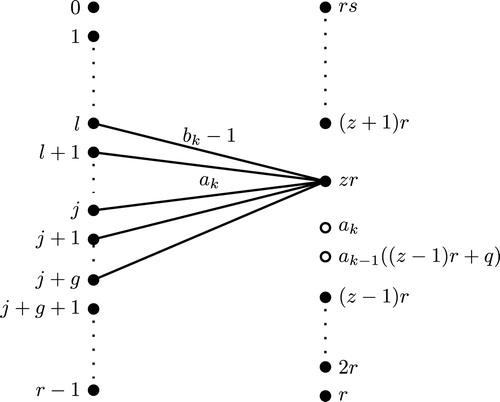
The number of missing vertex labels from to
is
, which is nothing but the number of all the labels in the interval
, for each
plus the number of labels that belong to the set
. Therefore,
. This would imply that the number of missing edge labels from
to
is also
. Hence the number of existing edges that are incident at the vertices
and the number of existing edges that are incident at the vertex
having the other end vertices
is equal to the number of possible edges that can be incident at the vertices
and the number of possible edges that can be incident at the vertex
having the other end vertices
minus the number of missing edge labels from
to
. Thus, the number of existing edges that are incident at the vertices
and the number of existing edges that are incident at the vertex
having the other end vertices
is
. These
edges of the tree
are nothing but the edges which are incident at the vertices
and edges which are incident at the vertex
from
to
. The graph induced by these
edges of
is a forest and it is denoted by
. Hence
(2)
(2) Now we count the number of vertices that belong to the forest
in
. To count, we consider the following two cases on the nature of the ends of the edge
. Note that, in the edge
of the rooted tree
, either
is a parent of
or
is a parent of
.
Case :
is a parent of
From construction of the tree , the structure of the tree
under this situation is given in .
Fig. 3 The structure of the bipartite tree under the Case
.
From , the vertices are the children of the vertices
. Hence, the forest
is the union of the subtrees of
rooted at
. Thus, from , the total number of vertices of
,
. This would imply that
. By Eq. (2),
. Thus,
. Hence
. Then from Observation 2.2, the label
is an existing vertex label. But by Case
, the label
is a missing vertex label. This is a contradiction. Hence, under this case our assumption
is wrong.
Case : When
is the parent of
Under this case, we consider the following two subcases.
Case : When
By our construction of the tree the structure of the tree
under this situation is given in . From , the vertices
are the children of the vertex
, where
.
Fig. 4 The structure of the bipartite tree under the Case
.
Then from , is the subtree rooted at the vertex
. Hence, the number of vertices of
,
. This would imply that
. By Eq. (2),
. Thus,
. Hence
. This implies that the label
is an existing vertex label. But by Case II, the label
is a missing vertex label which is a contradiction. Hence, under this case our assumption
is wrong.
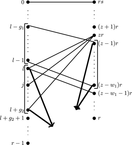
Case : When
By our construction of the tree the structure of the tree
under this situation is given in .
Fig. 5 The structure of the bipartite tree under the Case
.
From , the vertices are the children of the vertex
, where
. Then from ,
is the union of the subtrees rooted at
. The number of vertices in
,
. This would imply that
. By Eq. (2),
. This would imply that
. Hence
, which leads to a contradiction to the fact that the label
is a missing vertex label which lies in the interval
. Hence, under this case our assumption
is wrong.
Hence from all the cases, the assumption is wrong. Therefore,
. Hence, by induction,
, for every
,
. This means that the label
is non-negative for every
,
.
Since the current graph should contain all the vertex labels
. As
is a non-negative integer and as
,
must be a label of a vertex in that current graph
. □
Lemma 2.8
The graph obtained in the Embedding Algorithm is a graceful tree.
Proof
From Lemma 2.5, it is clear that after the execution of Step 5 of the Embedding Algorithm, we obtain the tree in which the vertices of
are labeled with distinct labels and the edges of
are also labeled with distinct labels. From the Embedding Algorithm, we observe that the graph
is obtained either after the complete execution of the Step 6.2 or after the complete execution of the Step 6.3.
Case 1: The graph obtained after the complete execution of the Step 6.2
As the Step 6.2 is executed only when , by Lemma 2.6, the tree
must be a star and it remains unchanged when Step 6.2 is executed. Consequently, the tree
should have been labeled as shown in . From , it is clear that the graph
is a tree with distinct vertex labels and distinct edge labels. More precisely, the vertex label set is
and the edge label set is
. Thus, by the definition of graceful labeling of the tree, the tree
is graceful.
Case 2: The graph obtained after the complete execution of the Step 6.3
In Step 6.3, the tree obtained after the execution of the Step 6.1 is taken as an input. The sets
and
are considered, where the elements of
and that of
are arranged in the increasing order respectively. Then for each
,
, the label
is found. By Lemma 2.7, the label
is non-negative and there always exists a vertex in the current graph
which has the label
. In the Step 6.3, for every
,
, a new vertex labeled with
is taken and it is joined with the existing vertex labeled
of the current graph
.
In Step 6.3, initially the graph is a tree and every execution of Step 6.3 a new vertex is added with existing vertex in
by a new pendant edge to the current graph
. Therefore the current graph
must be a tree. As
is always distinct for every
,
, and the vertex labels of the initial tree
are also distinct, the updated tree
contains distinct vertex labels in every execution. Further, note that in every execution of the Step 6.3, the distinct edge label
is obtained. As the edge labels of the initial tree
are also distinct, the final updated tree
contains distinct edge labels for all the edges. More precisely, the vertex label set of
are
and the edge label set of
are
. Thus, by the definition of graceful labeling of the tree, the tree
is graceful. □
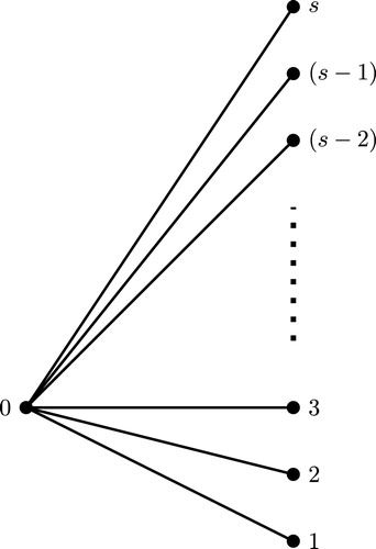
Fig. 6 The labeled tree obtained at the end of Step 6.2 of the embedding algorithm.
Theorem 2.9
The output graph obtained in the Step 7 of the Embedding Algorithm is a graceful unicyclic graph.
Proof
From the Embedding Algorithm, we observe that the output graph is obtained after the complete execution of the Step 7.1 or the output graph
is obtained after the complete execution of the Step 7.2.
Case 1: The graph obtained after the complete execution of the Step 7.1
Step 6.1 of the Embedding Algorithm is executed only when . Then by Lemma 2.6, the tree
is a star. Thus, after the execution of Step 6.2, the labeled tree
will be as shown in .
Fig. 7 The labeled tree after the execution of Step 6.2.
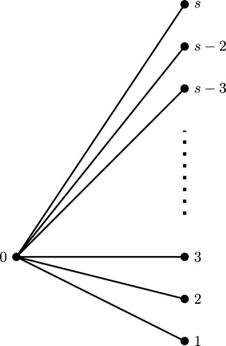
Thus, the labeled graph obtained after the execution of the Step 7.1 will be as shown in .
Fig. 8 The labeled graph obtained after the execution of Step 7.1.
It is clear from , the graph contains a unique cycle of length 3. Also, all the vertex labels are distinct and range over the set
and all the edge labels are also distinct and range over the set
. Then it follows from the definition of graceful labeling, the unicyclic graph
is graceful.
Case 2: The graph obtained after the complete execution of the Step 7.2, for
,
Here we consider two subcases depending on the value of .
Case 2.1:
Claim 1
The graph is unicyclic
In this case the input forest contains only one component,
. In Step 7.2.1, the fixed vertex
of
is joined with a new vertex
and this new vertex
is again joined with a chosen vertex
(which appear in the last level) of the tree
that contained in
as its subtree. Thus, after the execution of Step 7.2.1, the vertex set of the graph
is updated with a new vertex
with the label
and the edge set of
is also updated with two new edges having the labels
and
. (See .)
Fig. 9 The structure of the graceful unicyclic graph .
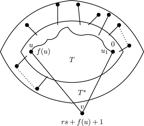
Fig. 10 The structure of the graceful unicyclic graph .
Since is a tree, the unique cycle connecting the vertex
of
to the vertex
of
which contained in
followed by the edge
and the edge
form a unique cycle of length
in
. Thus, the graph
is an unicyclic graph. By Lemma 2.8, the labels of all the vertices of the tree
are distinct and the labels of all the edges of the tree
are distinct. Therefore, after the execution of Step 7.2.1, the labels of the vertices of
,
are all distinct and edge labels of the edges of
,
are all distinct.
Claim 2
The graph is a graceful unicyclic graph
After the complete execution of Step 7.2.1.1, the vertex set of the graph is updated with
new pendant vertices which are labeled with
and the edge set of
is updated with
new pendant edges which get the labels
. Thus, after the complete execution of Step 7.2.1.1, the output graph
remains unicyclic.
After the complete execution of Step 7.2.1.1, in the output graph , the newly added vertices have distinct labels
that are all different from the labels of all the vertices of
and the newly added edges have distinct labels
that are all different from the labels of all the edges of
. Thus, the labels of all the vertices of
are distinct and the labels of all the edges of
are also distinct. More precisely, the set of labels of the vertices of
is
and the set of labels of the edges of
is
. Then it follows from the definition of graceful labeling, the unicyclic graph
is graceful.
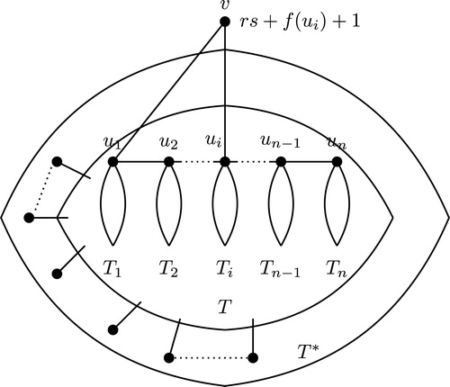
Case 2.2:
Claim 3
For every ,
, the graph
is unicyclic
In this case the input forest has at least two components. After the execution of Step 7.2, the fixed vertex of
that is contained in
as its subtree is joined with a new vertex
and this new vertex
is again joined with a fixed vertex
of
that is contained in
as its subtree. Thus, the vertex set of the graph
is updated with a new vertex
with the label
and the edge set of
is also updated with two new edges having the labels
and
. Since
is a tree, the unique cycle connecting the vertex
of
to the vertex
of
which is contained in
followed by the edge
and the edge
form a unique cycle of length
in
. Thus, the graph
is unicyclic. By Lemma 2.8, the labels of all the vertices of the tree
are distinct and the labels of all the edges of the tree
are distinct. Therefore, after the execution of Step 7.2.1, the labels of the vertices of
,
are all distinct and edge labels of the edges of
,
are all distinct. (See Fig. 10.)
Claim 4
The graph is a unicyclic graceful graph, for every
,
After the complete execution of Step 7.2.2.1, the vertex set of the graph is updated with
new pendant vertices which are labeled with
and the edge set of
is updated with
new pendant edges which get the labels
. After the complete execution of the Step 7.2.2.1, the output graph
remains as unicyclic.
After the complete execution of Step 7.2.2.1, in the output graph , the newly added vertices have distinct labels
that are all different from the labels of all the vertices of
and the newly added edges have distinct labels
that are all different from the labels of all the edges of
. Thus, the labels of all the vertices of
are distinct and the labels of all the edges of
are also distinct. More precisely, the set of labels of the vertices of
is
and the set of labels of the edges of
is
. Then it follows from the definition of graceful labeling, the unicyclic graph
is graceful. □
3 Discussion
From Theorem 2.9, we observe that the Embedding Algorithm generates distinct unicyclic graceful graphs and each unicyclic graph contains the given forest having
arbitrary trees
, for
as its subgraph. Also the Embedding Algorithm generates a unicyclic graceful graph with a fixed cycle length
if the input forest contains
components. All these unicyclic graphs obtained from Embedding Algorithm supports the Truszczynski’s conjecture Citation[6], that all unicyclic graphs except cycle
and
are graceful.
In this paper, we have embedded a given forest in a graceful tree as well as a graceful unicyclic graph. In this direction of graceful graph embedding, it would be interesting to explore the following questions.
| • | Is it possible to embed, a given unicyclic graph in a graceful unicyclic graph? | ||||
| • | What would be the minimum number of additional edges required for the embedding of a unicyclic graph into a graceful unicyclic graph? | ||||
Acknowledgments
The second author gratefully acknowledges Centre for Research, Anna University, Chennai, India for the financial support through the Anna Centenary Research Fellowship under the grant Ref: CR/ACRF/2014/40, Dated: 28.12.2013.
References
- WestD.B., Introduction to Graph Theorysecond ed.2001Prentice Hall of India
- G. Ringel, Problem 25, in: Theory of Graphs and its Applications, Proc. Symposium Smolenice, Prague, 1963, p. 162.
- KotzigA., Decompositions of a complete graph into 4k-gons Matematicky Casopis 151965 229–233(in Russian)
- RosaA., On certain valuations of the vertices of a graph, theory of graphs International Symposium, Rome, 19661967Gordon and Breach, N.Y. and Dunod Paris349–355
- GolombS.W., How to number a graphReadR.C.Graph Theory and Computing1972Academic PressNew York23–37
- TruszczynskiM., Graceful unicyclic graphs Demonstatio Math. 171984 377–387
- BarrientosC., Graceful graphs with pendant edges Australas. J. Combin. 332005 99–107
- BaggaJayArumurugamS., New classes of graceful unicyclic graphs Electron. Notes Discrete Math. 482015 27–32
- Figueroa-CentenoR.IchishimaR.Muntaner-BatleF.OshimaA., Gracefully cultivating trees on a cycle Electron. Notes Discrete Math. 482015 143–150
- GallianJ.A., A dynamic survey of graph labeling Electron. J. Combin. 202017 DS6
- AcharyaB.D., Construction of certain infinite families of graceful graphs from a given graceful graph Def. Sci. J. 321982 231–236
- SethuramanG.ElumalaiA., Packing of any set of graphs into a graceful/harmonious/elegant graph Ars Combin. 762005 297–301
- SethuramanG.RagukumarP.SlaterPeter J., Embedding an arbitrary tree in a graceful tree Bull. Malays. Math. Sci. Soc. 392016 341–360