Further results on Erdős–Faber–Lovász conjecture

Abstract

In 1972, Erdős–Faber–Lovász (EFL) conjectured that, if $\mathbf{H}$ is a linear hypergraph consisting of $n$ edges of cardinality $n$, then it is possible to color the vertices with $n$ colors so that no two vertices with the same color are in the same edge. In 1978, Deza, Erdös and Frankl had given an equivalent version of the same for graphs: Let $G={\bigcup }_{i=1}^n{A}_i$ denote a graph with $n$ complete graphs $A_1,A_2,$ $\dots ,A_n$, each having exactly $n$ vertices and have the property that every pair of complete graphs has at most one common vertex, then the chromatic number of $G$ is $n$. The clique degree $d^K\left(v\right)$ of a vertex $v$ in $G$ is given by $d^K\left(v\right)=\left|\{A_i:v\in V\left(A_i\right),1\le i\le n\}\right|$. In this paper we give a method for assigning colors to the graphs satisfying the hypothesis of the Erdős–Faber–Lovász conjecture and every $A_i$ ($1\le i\le n$) has atmost $\frac{n}{2}$ vertices of clique degree greater than one using Symmetric latin Squares and clique degrees of the vertices of $G$.

Keywords:

• Chromatic number
• Erdős–Faber–Lovász conjecture
• Symmetric latin square

1 Introduction

One of the famous conjectures in graph theory is Erdős–Faber–Lovász conjecture. It states that, if $\mathbf{H}$ is a linear hypergraph consisting of $n$ edges of cardinality $n$, then it is possible to color the vertices of $\mathbf{H}$ with $n$ colors so that no two vertices with the same color are in the same edge [1]. Erdős, in 1975, offered 50 USD [2,3] and in 1981, offered 500 USD [3,4] for the proof or disproof of the conjecture.

Vance Faber quoted: “In 1972, Paul Erdös, László Lovász and I got together at a tea party in Colorado. This was a continuation of the discussions we had a few weeks before in Columbus, Ohio, at a conference on hypergraphs. We talked about various conjectures for linear hypergraphs analogous to Vizing’s theorem for graphs. Finding tight bounds in general seemed difficult, so we created an elementary conjecture that we thought that it would be easy to prove. We called this the $n$ sets problem: given $n$ sets, no two of which meet more than once and each with $n$ elements, color the elements with $n$ colors so that each set contains all the colors. In fact, we agreed to meet the next day to write down the solution. Thirty-Eight years later, this problem is still unsolved in general”.

Chang and Lawler [5] presented a simple proof that the edges of a simple hypergraph on $n$ vertices can be colored with at most [1.5n-2] colors. Kahn [6] showed that the chromatic number of $\mathbf{H}$ is at most $n+o\left(n\right)$. Jackson et al. [7] proved that the conjecture is true when the partial hypergraph $S$ of $\mathbf{H}$ determined by the edges of size at least three can be ${\Delta }_S$-edge-colored and satisfies ${\Delta }_S\le 3$. In particular, the conjecture holds when $S$ is unimodular and ${\Delta }_S\le 3$. Viji Paul and Germina [8] established the truth of the conjecture for all linear hypergraphs on $n$ vertices with $\Delta \left(\mathbf{H}\right)\le \sqrt{n+\sqrt{n}+1}$ . Sanchez-Arroyo [9] proved the conjecture for dense hypergraphs. We consider the equivalent version of the conjecture for graphs given by Deza, Erdős and Frankl in 1978 [4,9–11].

Conjecture 1.1

Let $G={\bigcup }_{i=1}^n{A}_i$ denote a graph with $n$ complete graphs $(A_1,A_2,\dots ,A_n)$, each having exactly $n$ vertices and have the property that every pair of complete graphs has at most one common vertex, then the chromatic number of $G$ is $n$.

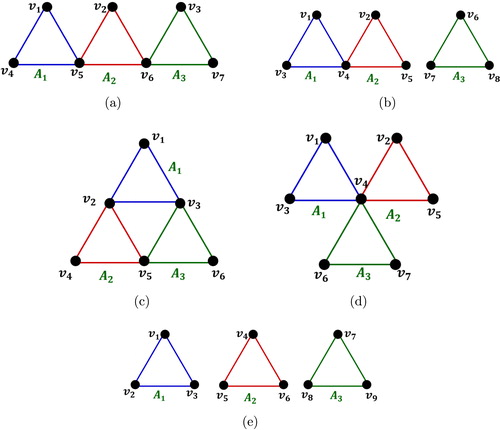
Example 1.2

Fig. 1 shows all the graphs for $n=3$ which are satisfying the hypothesis of Conjecture 1.1.

Fig. 1 All graphs satisfying the hypothesis of the conjecture for n $=$ 3.

Haddad & Tardif (2004) [12] introduced the problem with a story about seating assignment in committees: suppose that, in a university department, there are $k$ committees, each consisting of $k$ faculty members, and that all committees meet in the same room, which has $k$ chairs. Suppose also that at most one person belongs to the intersection of any two committees. Is it possible to assign the committee members to chairs in such a way that each member sits in the same chair for all the different committees to which he or she belongs? In this model of the problem, the faculty members correspond to graph vertices, committees correspond to complete graphs, and chairs correspond to vertex colors.

Definition 1.3

Let $G={\bigcup }_{i=1}^n{A}_i$ denote a graph with $n$ complete graphs $A_1,A_2$, $\dots ,A_n$, each having exactly $n$ vertices and the property that every pair of complete graphs has at most one common vertex. The clique degree $d^K\left(v\right)$ of a vertex $v$ in $G$ is given by $d^K\left(v\right)=\left|\{A_i:v\in V\left(A_i\right),1\le i\le n\}\right|$. The maximum clique degree ${\Delta }^K\left(G\right)$ of the graph $G$ is given by ${\Delta }^K\left(G\right)=ma{x}_{v\in V\left(G\right)}{d}^K\left(v\right)$.

From the above definition, one can observe that degree of a vertex in hypergraph is same as the clique degree of a vertex in a graph.

Definition 1.4

Let $G_1$ and $G_2$ be two vertex disjoint graphs, and let $x_1,x_2$ be two vertices of $G_1,G_2$ respectively. Then, the graph $G\left(x_1{x}_2\right)$ obtained by merging the vertices $x_1$ and $x_2$ into a single vertex is called the concatenation of $G_1$ and $G_2$ at the points $x_1$ and $x_2$ (see [13]).

Definition 1.5

A Latin Square is an $n\times n$ array containing $n$ different symbols such that each symbol appears exactly once in each row and once in each column. Moreover, a Latin Square of order $n$ is an $n\times n$ matrix $M=\left[m_{ij}\right]$ with entries from an $n$-set $V=\{1,2,\dots ,n\}$, where every row and every column is a permutation of V (see [14]). If the matrix $M$ is symmetric, then the Latin Square is called Symmetric Latin Square.

In this paper we give a method of coloring to the graph $G$ satisfying the hypothesis of the conjecture using a Symmetric Latin Square in the following steps:

•	Construct the graph $H_n$ having the minimum number of vertices among the graphs satisfying the hypothesis of the conjecture for given $n$
•	Construct any other graph satisfying the hypothesis of the conjecture for the same $n$.
•	We give a coloring to the graph $H_n$ with $n$ colors using a Symmetric Latin Square.
•	Extend the $n$-coloring of $H_n$ to the other graphs satisfying the hypothesis of Conjecture 1.1 for any given $n$.

2 Construction of $H_n$

We know that a symmetric $n\times n$ matrix is determined by $\frac{n(n+1)}{2}$ scalars. Using symmetric latin squares we give an $n$-coloring of $H_n$ constructed below.

Construction of $H_n$:

Let $n$ be a positive integer and $B_1,B_2,\dots ,B_n$ be $n$ copies of $K_n$. Let the vertex set $V\left(B_i\right)=\{a_{i,1},a_{i,2},a_{i,3},\dots ,a_{i,n}\}$, $1\le i\le n$.

Step 1. Let $H^1=B_1$.

Step 2. Consider the vertices $a_{1,2}$ of $H^1$ and $a_{2,1}$ of $B_2$. Let $b_{1,2}$ be the vertex obtained by the concatenation of the vertices $a_{1,2}$ and $a_{2,1}$. Let the resultant graph be $H^2$.

Step 3. Consider the vertices $a_{1,3}$, $a_{2,3}$ of $H^2$ and $a_{3,1}$, $a_{3,2}$ of $B_3$. Let $b_{1,3}$ be the vertex obtained by the concatenation of vertices $a_{1,3}$, $a_{3,1}$ and let $b_{2,3}$ be the vertex obtained by the concatenation of vertices $a_{2,3}$, $a_{3,2}$. Let the resultant graph be $H^3$.

Continuing in the similar way, at the $n$th step we obtain the graph $H^n=H_n$ (for the sake of convenience we take $H^n$ as $H_n$).

By the construction of $H_n$ one can observe the following:

1.	$H_n$ is a connected graph and also it is satisfying the hypothesis of Conjecture 1.1.
2.	$H_n$ has exactly $n$ vertices of clique degree one and $\frac{n(n-1)}{2}$ vertices of clique degree $2$ (each $B_i$ has exactly $(n-1)$ vertices of clique degree $2$ and one vertex of clique degree one, $1\le i\le n$).
3.	$H_n={\bigcup }_{i=1}^n{B}_i$, where $B_i=A_i$ and $B_i$, $B_j$ have exactly one common vertex for $1\le i<j\le n$.
4.	$H_n$ has exactly $\frac{n(n+1)}{2}$ vertices.
5.	One can observe that in a connected graph $G$ if clique degree increases the number of vertices also increases. From this it follows that, $H_n$ is the graph with minimum number of vertices satisfying the hypothesis of Conjecture 1.1. If all the vertices of $G$ are of clique degree one, then $G$ will have $n^2$ vertices. Thus, $\frac{n(n+1)}{2}\le \left|V\left(G\right)\right|\le n^2$.

Following example is an illustration of the graph $H_n$ for $n=4$

Example 2.1

Let $n=4$ and $B_1,B_2,B_3,B_4$ be the $4$ copies of $K_4$. Let the vertex set $V\left(B_i\right)=\{a_{i,1},a_{i,2},a_{i,3},a_{i,4}\}$, $1\le i\le 4$.

Step 1: Let $H^1=B_1$. The graph $H^1$ is shown in Fig. 2a.

Step 2: Consider the vertices $a_{1,2}$ of $H^1$ and $a_{2,1}$ of $B_2$. Let $b_{1,2}$ be the vertex obtained by the concatenation of vertices $a_{1,2}$, $a_{2,1}$. Let the resultant graph be $H^2$ as shown in Fig. 3b.

Step 3: Consider the vertices $a_{1,3}$, $a_{2,3}$ of $H^2$ and $a_{3,1}$, $a_{3,2}$ of $B_3$. Let $b_{1,3}$ be the vertex obtained by the concatenation of vertices $a_{1,3}$, $a_{3,1}$ and let $b_{2,3}$ be the vertex obtained by the concatenation of vertices $a_{2,3}$, $a_{3,2}$. Let the resultant graph be $H^3$ as shown in Fig. 4b.

Step 4: Consider the vertices $a_{1,4}$, $a_{2,4}$, $a_{3,4}$ of $H^3$ and $a_{4,1}$, $a_{4,2}$, $a_{4,3}$ of $B_4$. Let $b_{1,4}$ be the vertex obtained by the concatenation of vertices $a_{1,4}$, $a_{4,1}$, let $b_{2,4}$ be the vertex obtained by the concatenation of vertices $a_{2,4}$, $a_{4,2}$ and let $b_{3,4}$ be the vertex obtained by the concatenation of vertices $a_{3,4}$, $a_{4,3}$. Let the resultant graph be $H^4$ as shown in Fig. 5b.

Fig. 2 4 copies of $K_4$.

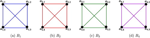
Fig. 3 Construction of $H^2$ from $H^1,B_2$.

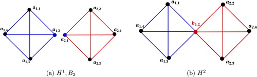
Fig. 4 Construction of $H^3$ from $H^2,B_3$.

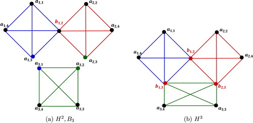
Fig. 5 Construction of $H^4$ from $H^3,B_4$.

Example 2.2

For $n=6$, the graph $H_6$ is shown in Fig. 6.

Fig. 6 $H_6$.

Lemma 2.3

If $G$ is a graph satisfying the hypothesis of Conjecture 1.1, then$G$ can be obtained from $H_n$,$n$ in$\mathbb{N}$.

Proof

Let $G$ be a graph satisfying the hypothesis of Conjecture 1.1. Let $b_X$ be the new labeling to the vertices $v$ of clique degree greater than $1$ in $G$, where $x=\{i$ : vertex $v$ is in $A_i\}$. Define $N_i=\{b_X:\left|X\right|=i\}$ for $i=2,3,\dots ,n$. Then the graph $G$ is constructed from $H_n$ as given below:

Step 1: For every common vertex $b_{i,j}$ in $H_n$ which is not in $N_2$, split the vertex $b_{i,j}$ into two vertices $u_{i,j},u_{j,i}$ such that vertex $u_{i,j}$ is adjacent only to the vertices of $B_i$ and the vertex $u_{j,i}$ is adjacent only to the vertices of $B_j$ in $H_n$.

Step 2: For every vertex $b_X$ in $N_i$ where $i=3,4,\dots ,n$, merge the vertices $u_{l_1,l_2}$, $u_{l_2,l_3}$, $\dots$, $u_{l_{m-1},l_m}$, $u_{l_m,l_1}$ into a single vertex $u_X$ in $H_n$ where $l_i\in X$ and $l_i<l_j$ for $i<j$.

Let $G^{\prime }$ be the graph obtained in Step 2. Let $V\left(B_i^{\prime }\right)$, $V\left(A_i^{\prime }\right)$ be the set of all clique degree 1 vertices of $B_i$ of $G^{\prime }$, $A_i$ of $G$ respectively, $1\le i\le n$. Thus, by splitting all the common vertices of $H_n$ which are not in $N_2$ and merging the vertices of $H_n$ corresponding to the vertices in $N_i,i\ge 3$, we get the graph $G^{\prime }$. One can observe that $\left|V\left(A_i^{\prime }\right)\right|=\left|V\left(B_i^{\prime }\right)\right|$, $1\le i\le n$. Define a function $f:V\left(G\right)\to V\left(G^{\prime }\right)$ by $$f\left(b_{i,j}\right)=b_{i,j}\text{for}{b}_{i,j}\in N_2$$$$f\left(b_{i_1,i_2,\dots i_k}\right)=u_{i_1,i_2,\dots i_k}\text{for}{b}_{i_1,i_2,\dots i_k}\in {\cup }_{i=3}^n{N}_i$$$$f{|}_{V\left(A_i^{\prime }\right)}=g_i(\text{any 1–1 map}{g}_i:V\left(A_i^{\prime }\right)\to V\left(B_i^{\prime }\right)),\text{for}1\le i\le n$$

One can observe that $f$ is an isomorphism from $G$ to $G^{\prime }$.■

From Lemma 2.3, one can observe that in $G$ there are at most $\frac{n(n-1)}{2}$ common vertices.

Following example is an illustration of the graph $G$ obtained from $H_n$ for $n=4$.

Example 2.4

Let $G$ be the graph shown in Fig. 7a.

Relabel the vertices of clique degree greater than one in $G$ by $b_A$ where $A=\{i:v\in A_i$ for $1\le i\le 4\}$. The labeled graph is shown in Fig. 7.

Let $N_i=\{b_x:\left|x\right|=i\}$ for $i=2,3,4$, then $N_2=\{b_{1,4},b_{2,4},b_{3,4}\}$, $N_3=\left\{b_{1,2,3}\right\}$.

Consider the graph $H_4$ as shown in Fig. 5b, then $V\left(H_4\right)=\{a_{1,1},a_{2,2},a_{3,3},a_{4,4},b_{1,2},b_{1,3},b_{1,4},b_{2,3},b_{2,4},b_{3,4}\}$ and common vertices of $H_4$ are $\{b_{1,2},b_{1,3},b_{1,4},b_{2,3},b_{2,4},b_{3,4}\}=A\left(say\right)$. Then $A\setminus N_2=\{b_{1,2},b_{1,3},b_{2,3}\}$. By the construction given in the proof of Lemma 2.3 we get,

Step 1: Since $A\setminus N_2\ne 0̸$, split the common vertices of $H_4$ which are not in $N_2$, as shown in Fig. 8.

Step 2: Since ${\cup }_{i=2}^4{N}_i=\left\{b_{1,2,3}\right\}\ne 0̸$, merge the vertices $u_{1,2},u_{2,3},u_{3,1}$ into a single vertex $u_{1,2,3}$, as shown in Fig. 9. Let the resultant graph be $G^{\prime }$.

The isomorphism $f:V\left(G\right)\to V\left(G^{\prime }\right)$ is given below. $$f\left(v_2\right)=a_{11}f\left(v_3\right)=u_{13}f\left(v_4\right)=u_{21}$$$$f\left(v_5\right)=a_{22}f\left(v_6\right)=u_{32}f\left(v_7\right)=a_{33}$$$$f\left(v_{1}1\right)=a_{44}f\left(b_{14}\right)=b_{14}f\left(b_{24}\right)=b_{24}$$$$f\left(b_{34}\right)=b_{34}f\left(b_{123}\right)=u_{123}$$

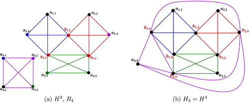
Fig. 7 Graph $G$, before and after relabeling the vertices.

Fig. 8 Splitting the common vertices of $H_4$ which are not in $N_2$.

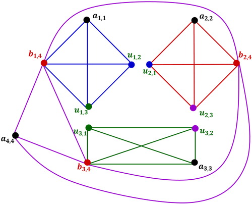
Fig. 9 Graph $G^{\prime }$.

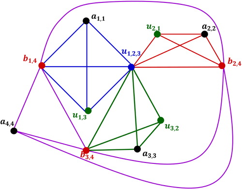
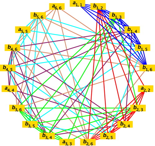
Fig. 10 A coloring of $H_6$ with six colors . (For interpretation of the references to color in this figure legend, the reader is referred to the web version of this article.)

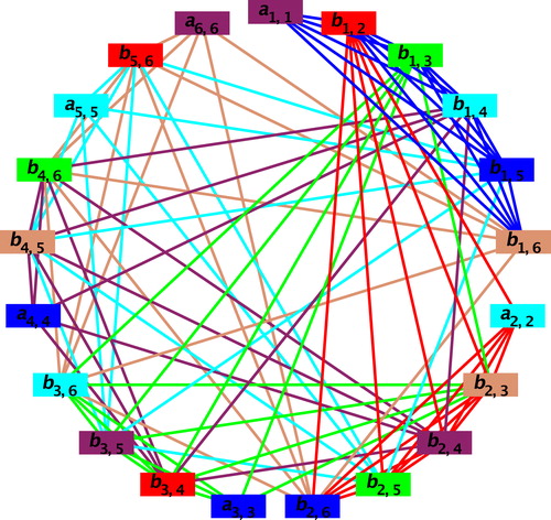
Fig. 11 Graph $G$: before and after relabeling the vertices.

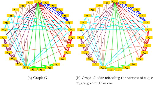
Fig. 12 Graph $\hat{H}$.

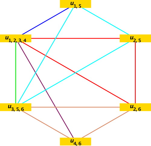
Fig. 13 The graphs $\hat{H}$ and $G$, after colors have been assigned to their vertices . (For interpretation of the references to color in this figure legend, the reader is referred to the web version of this article.)

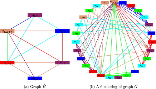
Fig. 14 Graph $G$: before and after relabeling the vertices.

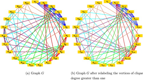
Fig. 15 Graph $\hat{H}$.

Fig. 16 The graphs $\hat{H}$ and $G$, after colors have been assigned to their vertices . (For interpretation of the references to color in this figure legend, the reader is referred to the web version of this article.)

3 Coloring of $H_n$

Lemma 3.1

The chromatic number of $H_n$ is $n$.

Proof

Let $H_n$ be the graph defined as above. Let $M$ (given below) be an $n\times n$ matrix in which an entry $m_{ij}=b_{ij}$, be a vertex of $H_n$, belongs to both $B_i,B_j$ for $i\ne j$ and $m_{ii}=a_{ii}$ be the vertex of $H_n$ which belongs to $B_i$. i.e., $$\mathrm{M}=\left(\begin{array}{ccccc}\hfill a_{11}\hfill & \hfill b_{12}\hfill & \hfill b_{13}\hfill & \hfill \dots \hfill & \hfill b_{1n}\hfill \\ \hfill b_{12}\hfill & \hfill a_{22}\hfill & \hfill b_{23}\hfill & \hfill \dots \hfill & \hfill b_{2n}\hfill \\ \hfill b_{13}\hfill & \hfill b_{23}\hfill & \hfill a_{33}\hfill & \hfill \dots \hfill & \hfill b_{3n}\hfill \\ \hfill ⋮\hfill & \hfill ⋮\hfill & \hfill ⋮\hfill & \hfill \ddots \hfill & \hfill ⋮\hfill \\ \hfill b_{1n}\hfill & \hfill b_{2n}\hfill & \hfill b_{3n}\hfill & \hfill \dots \hfill & \hfill a_{nn}\hfill \end{array}\right).$$

Clearly $M$ is a symmetric matrix. We know that, for every $n$ in $\mathbb{N}$ there is a Symmetric Latin Square (see [15]) of order $n\times n$. Bryant and Rodger [16] gave a necessary and sufficient condition for the existence of an $(n-1)$-edge coloring of $K_n$ (n even), and $n$-edge coloring of $K_n$ (n odd) using Symmetric Latin Squares. Let $v_1,v_2,\dots ,v_n$ be the vertices of $K_n$ and $e_{ij}$ be the edge joining the vertices $v_i$ and $v_j$ of $K_n$, where $i<j$, then arrange the edges of $K_n$ in the matrix form $A=\left[a_{ij}\right]$ where $a_{ij}=e_{ij}$, $a_{ji}=e_{ij}$ for $i<j$ and $a_{ii}=0$ for $1\le i\le n$, we have $A=\left(\begin{array}{ccccc}\hfill 0\hfill & \hfill e_{12}\hfill & \hfill e_{13}\hfill & \hfill \dots \hfill & \hfill e_{1n}\hfill \\ \hfill e_{12}\hfill & \hfill 0\hfill & \hfill e_{23}\hfill & \hfill \dots \hfill & \hfill e_{2n}\hfill \\ \hfill e_{13}\hfill & \hfill e_{23}\hfill & \hfill 0\hfill & \hfill \dots \hfill & \hfill e_{3n}\hfill \\ \hfill ⋮\hfill & \hfill ⋮\hfill & \hfill ⋮\hfill & \hfill \ddots \hfill & \hfill ⋮\hfill \\ \hfill e_{1n}\hfill & \hfill e_{2n}\hfill & \hfill e_{3n}\hfill & \hfill \dots \hfill & \hfill 0\hfill \end{array}\right)$and let $V$ be a matrix given by $V=\left(\begin{array}{ccccc}\hfill v_1\hfill & \hfill 0\hfill & \hfill 0\hfill & \hfill \dots \hfill & \hfill 0\hfill \\ \hfill 0\hfill & \hfill v_2\hfill & \hfill 0\hfill & \hfill \dots \hfill & \hfill 0\hfill \\ \hfill 0\hfill & \hfill 0\hfill & \hfill v_3\hfill & \hfill \dots \hfill & \hfill 0\hfill \\ \hfill ⋮\hfill & \hfill ⋮\hfill & \hfill ⋮\hfill & \hfill \ddots \hfill & \hfill ⋮\hfill \\ \hfill 0\hfill & \hfill 0\hfill & \hfill 0\hfill & \hfill \dots \hfill & \hfill v_n\hfill \end{array}\right)$. Then, define a matrix $A^{\prime }$ as $$A^{\prime }=A+V=\left(\begin{array}{ccccc}\hfill v_1\hfill & \hfill e_{12}\hfill & \hfill e_{13}\hfill & \hfill \dots \hfill & \hfill e_{1n}\hfill \\ \hfill e_{12}\hfill & \hfill v_2\hfill & \hfill e_{23}\hfill & \hfill \dots \hfill & \hfill e_{2n}\hfill \\ \hfill e_{13}\hfill & \hfill e_{23}\hfill & \hfill v_3\hfill & \hfill \dots \hfill & \hfill e_{3n}\hfill \\ \hfill ⋮\hfill & \hfill ⋮\hfill & \hfill ⋮\hfill & \hfill \ddots \hfill & \hfill ⋮\hfill \\ \hfill e_{1n}\hfill & \hfill e_{2n}\hfill & \hfill e_{3n}\hfill & \hfill \dots \hfill & \hfill v_n\hfill \end{array}\right).$$

Let $C=\left[c_{ij}\right]$ be a matrix where $c_{ij}$ ($i\ne j$), is the color of $e_{ij}$ (i.e., $c_{ij}=c\left(e_{ij}\right)$) and $c_{ii}$ is the color of $v_i$. We call $C$ as the color matrix of $A^{\prime }$. Then $C$ is the Symmetric Latin Square (see [16]). As the elements of $M$ are the vertices of $H_n$, one can assign the colors to the vertices of $H_n$ from the color matrix $C$, by the color $c_{ij}$, for $i,j=1,2,\dots ,n$ and $i\ne j$ to the vertex $b_{ij}$ in $H_n$ and the color $c_{ii}$, for $i=1,2,\dots n$ to the vertex $a_{ii}$ in $H_n$. Hence $H_n$ is $n$ colorable.■

$H_n$ is the graph satisfying the hypothesis of Conjecture 1.1. By using the coloring of $H_n$ which is the graph satisfying the hypothesis of Conjecture 1.1 we extend the $n$-coloring of all possible graphs $G$ satisfying the hypothesis of Conjecture 1.1.

The following example is an illustration of assigning colors to the graph $H_n$ for $n=6$.

Example 3.2

Consider the graph $H_6$ as shown in Fig. 6. The corresponding Symmetric Latin Square $C$ of order 6 × 6 is given below: $$C=\left(\begin{array}{cccccc}\hfill 6\hfill & \hfill 1\hfill & \hfill 2\hfill & \hfill 3\hfill & \hfill 4\hfill & \hfill 5\hfill \\ \hfill 1\hfill & \hfill 3\hfill & \hfill 5\hfill & \hfill 6\hfill & \hfill 2\hfill & \hfill 4\hfill \\ \hfill 2\hfill & \hfill 5\hfill & \hfill 4\hfill & \hfill 1\hfill & \hfill 6\hfill & \hfill 3\hfill \\ \hfill 3\hfill & \hfill 6\hfill & \hfill 1\hfill & \hfill 4\hfill & \hfill 5\hfill & \hfill 2\hfill \\ \hfill 4\hfill & \hfill 2\hfill & \hfill 6\hfill & \hfill 5\hfill & \hfill 3\hfill & \hfill 1\hfill \\ \hfill 5\hfill & \hfill 4\hfill & \hfill 3\hfill & \hfill 2\hfill & \hfill 1\hfill & \hfill 6\hfill \end{array}\right).$$

Assign the six colors to the graph $H_6$ using the above Symmetric Latin Square as follows:

Assign the color $c_{i,j}$ (where $c_{i,j}$ denotes the value at the $(i,j)$th entry in the color matrix $C$) for $i\ne j$ and $i,j=1,2,\dots ,6$ to the vertex $b_{i,j}$ in $H_6$, and assign the color $c_{i,i}$ (where $c_{i,i}$ denotes the value at the $(i,i)$th entry in the color matrix $C$) for $i=1,2,\dots ,6$ to the vertex $a_{ii}$ in $H_6$. The colors Red, Green, Cyan, Blue, Tan, Maroon in Fig. 10 corresponds to the numbers 1, 2, 3, 4, 5, 6 respectively in the matrix $C$.

Then one can verify that the resultant graph is $6$ colorable as shown in Fig. 10.

4 Coloring of $G$

Let $G$ be the graph satisfying the hypothesis of Conjecture 1.1. Let $\hat{H}$ be the graph obtained by removing the vertices of clique degree one from graph $G$. i.e. $\hat{H}$ is the induced subgraph of $G$ having all the common vertices of $G$.

Method for assigning colors to graph $G$ satisfying the hypothesis of Conjecture 1.1 and every $A_i$ ($1\le i\le n$) has atmost $\frac{n}{2}$ vertices of clique degree greater than one:

Let $G$ be a graph satisfying the hypothesis of Conjecture 1.1 and every $A_i$ ($1\le i\le n$) has atmost $\frac{n}{2}$ vertices of clique degree greater than one. Let $\hat{H}$ be the induced subgraph of $G$ consisting of the vertices of clique degree greater than one in $G$. For every vertex $v$ of clique degree greater than one in $G$, label the vertex $v$ by $u_A$ where $A=\{i:v\in A_i;i=1,2,\dots ,n\}$. Define $X=\{b_{i,j}:A_i\cap A_j=0̸\}$, $X_i=\{v\in G:d^K\left(v\right)=i\}$ for $i=1,2,\dots ,m$.

Let $1,2,\dots ,n$ be the $n$-colors and $C$ be the color matrix (of size $n\times n$) as defined in the proof of Lemma 3.1. The following construction applied on the color matrix $C$, gives a modified color matrix $C_M$, using which we assign the colors to the graph $\hat{H}$. Then this coloring can be extended to the graph $G$. Construct a new color matrix $C_1$ by putting $c_{i,j}=0,c_{j,i}=0$ for every $b_{i,j}$ in $X$. Also, let $c_{i,i}=0$ for each $i=1,2,\dots ,n$.

Let $T={\cup }_{i=3}^n{X}_i$, $P=0̸$, $T^{\prime \prime }=X_2$ and $P^{\prime \prime }=0̸$.

Step 1:	If $T=0̸$, let $C_m$ be the color matrix obtained in Step 4 and go to Step 5. Otherwise, choose a vertex $u_{i_1,i_2,\dots ,i_m}$ from $T$, where $i_1<i_2<\cdots <i_m$, and then choose $\left(\genfrac{}{}{0ex}{}{m}{2}\right)$ vertices $b_{i_1,i_2}$, $b_{i_1,i_3}$, $\dots$, $b_{i_1,i_m}$, $b_{i_2,i_3}$, $\dots$, $b_{i_{m-1},i_m}$ from $V\left(H_n\right)$ corresponding to the set $\{i_1,i_2,\dots ,i_m\}$. Take $T^{\prime }=\{b_{i_1,i_2},b_{i_1,i_3},\dots ,b_{i_1,i_m},b_{i_2,i_3},\dots ,b_{i_{m-1},i_m}\}$ and $P^{\prime }=0̸$. Let $T_1^{\prime }=\{b_{i,j}:b_{i,j}\in T^{\prime },c\left(b_{i,j}\right)$ appear more than once in the $i$th row or $j$th column in $C\}$ and $T_2^{\prime }=\{b_{i,j}:b_{i,j}\in T^{\prime },c\left(b_{i,j}\right)$ appear exactly once in the $i$th row and $j$th column in $C\}$. If $T_1^{\prime }\ne 0̸$, choose a vertex $b_{s,t}$ from $T_1^{\prime }$, otherwise choose a vertex $b_{s,t}$ from $T_2^{\prime }$. Then add the vertex $b_{s,t}$ to $P^{\prime }$ and remove it from $T^{\prime }$. Go to Step 2.
Step 2:	If $T_2^{\prime }\ne 0̸$, go to Step 3. Otherwise, choose a vertex $b_{i_{m-1},i_m}$ from $T_1^{\prime }$. Let $A=\{c_{i,j}:c_{i,j}\ne 0;i=i_{m-1},1\le j\le n\}$, $B=\{c_{i,j}:c_{i,j}\ne 0;j=i_m,1\le i\le n\}$. If $|A\cap B|<n$, then construct a new color matrix $C_2$, replacing $c_{i_{m-1},i_m}$, $c_{i_m,i_{m-1}}$ by $x$, where $x\in \{1,2,\dots ,n\}\setminus A\cup B$. Then add the vertex $b_{i_{m-1},i_m}$ to $T_2^{\prime }$ and remove it from $T_1^{\prime }$. Go to Step 3. Otherwise choose a color $x$ which appears exactly once either in $i_{m-1}$th row or in $i_m$th column of the color matrix and construct a new color matrix $C_2$ replacing $c_{i_{m-1},i_m}$, $c_{i_m,i_{m-1}}$ by $x$. Then add the vertex $b_{i_{m-1},i_m}$ to $T_2^{\prime }$ and remove it from $T_1^{\prime }$. Go to Step 3.
Step 3:	If $T^{\prime }=0̸$, then add the vertex $u_{i_1,i_2,\dots ,i_m}$ to $P$ and remove it from $T$, go to Step 1. Otherwise, if $T^{\prime }\cap T_1^{\prime }\ne 0̸$ choose a vertex $b_{i,j}$ from $T^{\prime }\cap T_1^{\prime }$, if not choose a vertex $b_{i,j}$ from $T^{\prime }\cap T_2^{\prime }$. Go to Step 4.
Step 4:	Let $c\left(b_{i,j}\right)=x,c\left(b_{s,t}\right)=y$. If $c\left(b_{i,j}\right)=c\left(b_{s,t}\right)$, then add the vertex $b_{i,j}$ to $P^{\prime }$ and remove it from $T^{\prime }$. Go to Step 3. Otherwise, let $A=\{c_{l,m}:c_{l,m}=x\}$, $B=\{c_{l,m}:c_{l,m}=y\}\setminus \{c_{l,m},c_{m,l}:b_{l,m}\in P^{\prime },l<m\}$. Construct a new color matrix $C_3$ by putting $c_{l,m}=y$ for every $c_{l,m}$ in $A$ and $c_{l,m}=x$ for every $c_{l,m}$ in B. Then add the vertex $b_{i,j}$ to $P^{\prime }$ and remove it from $T^{\prime }$. Go to Step 3.
Step 5:	If $T^{\prime \prime }=0̸$, consider $C_M=C_{m_1}$ stop the process. Otherwise, choose a vertex $u_{i,j}$ from $T^{\prime \prime }$ and go to Step 6.
Step 6:	If $c_{i,j}$ appears exactly once in both $i$th row and $j$th column of the color matrix $C_m$, then add the vertex $b_{i,j}$ to $P^{\prime \prime }$ and remove it from $T^{\prime \prime }$, go to Step 5. Otherwise, let $A=\{c_{i,j}:c_{i,j}\ne 0;1\le j\le n\}$, $B=\{c_{i,j}:c_{i,j}\ne 0;1\le i\le n\}$. Construct a new color matrix $C_{m_1}$ by putting $x$ in $c_{i,j}$, $c_{j,i}$ where $x\in \{1,2,\dots ,n\}\setminus A\cup B$ (since every $A_i$ ($1\le i\le n$) has atmost $\frac{n}{2}$ vertices of clique degree greater than one, $|A\cup B|<n$). Then add the vertex $u_{i,j}$ to $P^{\prime \prime }$ and remove it from $T^{\prime \prime }$, go to Step 5.

Thus, in step 6, we get the modified color matrix $C_M$. Then, color the vertex $v$ of $\hat{H}$ by $c_{i,j}$ of $C_M$, whenever $v\in A_i\cap A_j$. Then, extend the coloring of $\hat{H}$ to $G$ by assigning the remaining colors which are not used for $A_i$ from the set of $n$-colors, to the vertices of clique degree one in $A_i$, $1\le i\le n$. Thus $G$ is $n$-colorable.

Remark 4.1

One can see that the above method covers the following cases:

1.	$G$ has no clique degree $2$ vertices.
2.	$G$ has atmost $\frac{n}{2}$ vertices of clique degree greater than one in each $A_i$, $1\le i\le n$.

Following is an example illustrating the above method.

Example 4.2

Let $G$ be the graph shown in Fig. 11a.

Let $V\left(A_1\right)=\{v_1,v_2,v_3,v_4,v_5,v_6\}$, $V\left(A_2\right)=\{v_1,v_7,v_8,v_9,v_{10},v_{11}\}$,

$V\left(A_3\right)=\{v_1,v_{12},v_{13},v_{14},v_{15},v_{16}\}$, $V\left(A_4\right)=\{v_1,v_{17},v_{18},v_{19},v_{20},v_{21}\}$,

$V\left(A_5\right)=\{v_6,v_7,v_{16},v_{22},v_{23},v_{24}\}$, $V\left(A_6\right)=\{v_9,v_{16},v_{19},v_{25},v_{26},v_{27}\}$.

Relabel the vertices of clique degree greater than one in $G$ by $u_A$ where $A=\{i:v\in A_i\text{for}1\le i\le 6\}$. The labeled graph is shown in Fig. 11b. Fig. 12 is the graph $\hat{H}$, where $\hat{H}$ is obtained by removing the vertices of clique degree 1 from $G$.

Let $X=\{b_{ij}:A_i\cap A_j=0̸\}=\{b_{1,6},b_{4,5}\}$, $$X_1=\{v\in G:d^K\left(v\right)=1\}=\{v_2,v_3,v_5,v_8,v_{10},v_{11},v_{12},v_{13},v_{14},v_{15},v_{17},v_{18},v_{20},v_{21},v_{22},v_{23},v_{24},v_{25},v_{26},v_{27}\},$$ $$X_2=\{v\in G:d^K\left(v\right)=2\}=\{v_6,v_7,v_9,v_{19}\}=\{u_{1,5},u_{2,5},u_{2,6},u_{4,6}\},$$ $$X_3=\{v\in G:d^K\left(v\right)=3\}=\left\{v_{16}\right\}=\left\{u_{3,5,6}\right\},$$

and $X_4=\{v\in G:d^K\left(v\right)=4\}=\left\{v_1\right\}=\left\{u_{1,2,3,4}\right\}$.

Let 1, 2, $\dots$, 6 be the six colors and $C=\left(\begin{array}{cccccc}\hfill 6\hfill & \hfill 1\hfill & \hfill 2\hfill & \hfill 3\hfill & \hfill 4\hfill & \hfill 5\hfill \\ \hfill 1\hfill & \hfill 3\hfill & \hfill 5\hfill & \hfill 6\hfill & \hfill 2\hfill & \hfill 4\hfill \\ \hfill 2\hfill & \hfill 5\hfill & \hfill 4\hfill & \hfill 1\hfill & \hfill 6\hfill & \hfill 3\hfill \\ \hfill 3\hfill & \hfill 6\hfill & \hfill 1\hfill & \hfill 4\hfill & \hfill 5\hfill & \hfill 2\hfill \\ \hfill 4\hfill & \hfill 2\hfill & \hfill 6\hfill & \hfill 5\hfill & \hfill 3\hfill & \hfill 1\hfill \\ \hfill 5\hfill & \hfill 4\hfill & \hfill 3\hfill & \hfill 2\hfill & \hfill 1\hfill & \hfill 6\hfill \end{array}\right)$

be the color matrix (as well as symmetric latin square) of order 6 × 6.

Consider the sets $T=X_3\cup X_4=\{u_{3,5,6},u_{1,2,3,4}\}$, $T^{\prime \prime }=X_2=\{u_{1,5},u_{2,5},u_{2,6},u_{4,6}\}$, $P=0̸$ and $P^{\prime \prime }=0̸$. Then, by applying the aforementioned method we get a new color matrix $C_1$ by putting $c_{i,j}=0$, $c_{j,i}=0$ for every $b_{i,j}$ in $X$ and $c_{i,i}=0$ for each $i=1,2,\dots ,6$ and go to Step 1. $$C_1=\left(\begin{array}{cccccc}\hfill 0\hfill & \hfill 1\hfill & \hfill 2\hfill & \hfill 3\hfill & \hfill 4\hfill & \hfill 0\hfill \\ \hfill 1\hfill & \hfill 0\hfill & \hfill 5\hfill & \hfill 6\hfill & \hfill 2\hfill & \hfill 4\hfill \\ \hfill 2\hfill & \hfill 5\hfill & \hfill 0\hfill & \hfill 1\hfill & \hfill 6\hfill & \hfill 3\hfill \\ \hfill 3\hfill & \hfill 6\hfill & \hfill 1\hfill & \hfill 0\hfill & \hfill 0\hfill & \hfill 2\hfill \\ \hfill 4\hfill & \hfill 2\hfill & \hfill 6\hfill & \hfill 0\hfill & \hfill 0\hfill & \hfill 1\hfill \\ \hfill 0\hfill & \hfill 4\hfill & \hfill 3\hfill & \hfill 2\hfill & \hfill 1\hfill & \hfill 0\hfill \end{array}\right)$$

Step 1: Since $T\ne 0̸$, choose the vertex $u_{1,2,3,4}$ from $T$. Let $T^{\prime }=\{b_{1,2},b_{1,3},b_{1,4},b_{2,3},b_{2,4},b_{3,4}\}$ and $P^{\prime }=0̸$, then $T_1^{\prime }=0̸$ and $T_2^{\prime }=T^{\prime }$. Since $T_1^{\prime }=0̸$, choose the vertex $b_{2,4}$ from $T_2^{\prime }$, add it to $P^{\prime }$ and remove it from $T^{\prime }$. Then $T^{\prime }=\{b_{1,2},b_{1,3},b_{1,4},b_{2,3},b_{3,4}\}$ and $P^{\prime }=\left\{b_{2,4}\right\}$. Go to step 2.

Step 2: Since $T_2^{\prime }\ne 0̸$, go to step 3.

Step 3: Since $T^{\prime }\ne 0̸$ and $T^{\prime }\cap T_1^{\prime }=0̸$, choose the vertex $b_{1,2}$ from $T^{\prime }\cap T_2^{\prime }$ and go to step 4.

Step 4: Since $c\left(b_{1,2}\right)=1$, $c\left(b_{2,4}\right)=6$ and $c\left(b_{1,2}\right)\ne c\left(b_{2,4}\right)$, interchange 1, 6 in the matrix $C_1$ except the color of $b_{2,4}$. Add the vertex $b_{1,2}$ to $P^{\prime }$ and remove it from $T^{\prime }$. Then $$C_2=\left(\begin{array}{cccccc}\hfill 0\hfill & \hfill 6\hfill & \hfill 2\hfill & \hfill 3\hfill & \hfill 4\hfill & \hfill 0\hfill \\ \hfill 6\hfill & \hfill 0\hfill & \hfill 5\hfill & \hfill 6\hfill & \hfill 2\hfill & \hfill 4\hfill \\ \hfill 2\hfill & \hfill 5\hfill & \hfill 0\hfill & \hfill 6\hfill & \hfill 1\hfill & \hfill 3\hfill \\ \hfill 3\hfill & \hfill 6\hfill & \hfill 6\hfill & \hfill 0\hfill & \hfill 0\hfill & \hfill 2\hfill \\ \hfill 4\hfill & \hfill 2\hfill & \hfill 1\hfill & \hfill 0\hfill & \hfill 0\hfill & \hfill 6\hfill \\ \hfill 0\hfill & \hfill 4\hfill & \hfill 3\hfill & \hfill 2\hfill & \hfill 6\hfill & \hfill 0\hfill \end{array}\right),$$

$T^{\prime }=\{b_{1,3},b_{1,4},b_{2,3},b_{3,4}\}$ and $P^{\prime }=\{b_{1,2},b_{2,4}\}$. Go to step 3.

Step 3: Since $T^{\prime }\ne 0̸$ and $T^{\prime }\cap T_1^{\prime }=0̸$, choose the vertex $b_{1,3}$ from $T^{\prime }\cap T_2^{\prime }$ and go to step 4.

Step 4: Since $c\left(b_{1,3}\right)=2$, $c\left(b_{2,4}\right)=6$ and $c\left(b_{1,3}\right)\ne c\left(b_{2,4}\right)$, interchange 2, 6 in the matrix $C_2$ except the color of $b_{1,2},b_{2,4}$. Add the vertex $b_{1,3}$ to $P^{\prime }$ and remove it from $T^{\prime }$. Then $$C_3=\left(\begin{array}{cccccc}\hfill 0\hfill & \hfill 6\hfill & \hfill 6\hfill & \hfill 3\hfill & \hfill 4\hfill & \hfill 0\hfill \\ \hfill 6\hfill & \hfill 0\hfill & \hfill 5\hfill & \hfill 6\hfill & \hfill 6\hfill & \hfill 4\hfill \\ \hfill 6\hfill & \hfill 5\hfill & \hfill 0\hfill & \hfill 2\hfill & \hfill 1\hfill & \hfill 3\hfill \\ \hfill 3\hfill & \hfill 6\hfill & \hfill 2\hfill & \hfill 0\hfill & \hfill 0\hfill & \hfill 6\hfill \\ \hfill 4\hfill & \hfill 6\hfill & \hfill 1\hfill & \hfill 0\hfill & \hfill 0\hfill & \hfill 2\hfill \\ \hfill 0\hfill & \hfill 4\hfill & \hfill 3\hfill & \hfill 6\hfill & \hfill 2\hfill & \hfill 0\hfill \end{array}\right),$$

$T^{\prime }=\{b_{1,4},b_{2,3},b_{3,4}\}$ and $P^{\prime }=\{b_{1,2},b_{1,3},b_{2,4}\}$. Go to step 3.

Step 3: Since $T^{\prime }\ne 0̸$ and $T^{\prime }\cap T_1^{\prime }=0̸$, choose the vertex $b_{1,4}$ from $T^{\prime }\cap T_2^{\prime }$ and go to step 4.

Step 4: Since $c\left(b_{1,4}\right)=3$, $c\left(b_{2,4}\right)=6$ and $c\left(b_{1,4}\right)\ne c\left(b_{2,4}\right)$, interchange 3, 6 in the matrix $C_3$ except the color of $b_{1,2},b_{1,3},b_{2,4}$. Add the vertex $b_{1,4}$ to $P^{\prime }$ and remove it from $T^{\prime }$. Then $$C_4=\left(\begin{array}{cccccc}\hfill 0\hfill & \hfill 6\hfill & \hfill 6\hfill & \hfill 6\hfill & \hfill 4\hfill & \hfill 0\hfill \\ \hfill 6\hfill & \hfill 0\hfill & \hfill 5\hfill & \hfill 6\hfill & \hfill 3\hfill & \hfill 4\hfill \\ \hfill 6\hfill & \hfill 5\hfill & \hfill 0\hfill & \hfill 2\hfill & \hfill 1\hfill & \hfill 6\hfill \\ \hfill 6\hfill & \hfill 6\hfill & \hfill 2\hfill & \hfill 0\hfill & \hfill 0\hfill & \hfill 3\hfill \\ \hfill 4\hfill & \hfill 3\hfill & \hfill 1\hfill & \hfill 0\hfill & \hfill 0\hfill & \hfill 2\hfill \\ \hfill 0\hfill & \hfill 4\hfill & \hfill 6\hfill & \hfill 3\hfill & \hfill 2\hfill & \hfill 0\hfill \end{array}\right),$$

$T^{\prime }=\{b_{2,3},b_{3,4}\}$ and $P^{\prime }=\{b_{1,2},b_{1,3},b_{1,4},b_{2,4}\}$. Go to step 3.

Step 3: Since $T^{\prime }\ne 0̸$ and $T^{\prime }\cap T_1^{\prime }=0̸$, choose the vertex $b_{2,3}$ from $T^{\prime }\cap T_2^{\prime }$ and go to step 4.

Step 4: Since $c\left(b_{2,3}\right)=5$, $c\left(b_{2,4}\right)=6$ and $c\left(b_{2,3}\right)\ne c\left(b_{2,4}\right)$, interchange 5, 6 in the matrix $C_4$ except the color of $b_{1,2},b_{1,3},b_{1,4},b_{2,4}$. Add the vertex $b_{2,3}$ to $P^{\prime }$ and remove it from $T^{\prime }$. Then $$C_5=\left(\begin{array}{cccccc}\hfill 0\hfill & \hfill 6\hfill & \hfill 6\hfill & \hfill 6\hfill & \hfill 4\hfill & \hfill 0\hfill \\ \hfill 6\hfill & \hfill 0\hfill & \hfill 6\hfill & \hfill 6\hfill & \hfill 3\hfill & \hfill 4\hfill \\ \hfill 6\hfill & \hfill 6\hfill & \hfill 0\hfill & \hfill 2\hfill & \hfill 1\hfill & \hfill 5\hfill \\ \hfill 6\hfill & \hfill 6\hfill & \hfill 2\hfill & \hfill 0\hfill & \hfill 0\hfill & \hfill 3\hfill \\ \hfill 4\hfill & \hfill 3\hfill & \hfill 1\hfill & \hfill 0\hfill & \hfill 0\hfill & \hfill 2\hfill \\ \hfill 0\hfill & \hfill 4\hfill & \hfill 5\hfill & \hfill 3\hfill & \hfill 2\hfill & \hfill 0\hfill \end{array}\right),$$

$T^{\prime }=\left\{b_{3,4}\right\}$ and $P^{\prime }=\{b_{1,2},b_{1,3},b_{1,4},b_{2,3},b_{2,4}\}$. Go to step 3.

Step 3: Since $T^{\prime }\ne 0̸$ and $T^{\prime }\cap T_1^{\prime }=0̸$, choose the vertex $b_{3,4}$ from $T^{\prime }\cap T_2^{\prime }$ and go to step 4.

Step 4: Since $c\left(b_{3,4}\right)=2$, $c\left(b_{2,4}\right)=6$ and $c\left(b_{3,4}\right)\ne c\left(b_{2,4}\right)$, interchange 2, 6 in the matrix $C_5$ except the color of $b_{1,2},b_{1,3},b_{1,4},b_{2,3},b_{2,4}$. Add the vertex $b_{3,4}$ to $P^{\prime }$ and remove it from $T^{\prime }$. Then $$C_6=\left(\begin{array}{cccccc}\hfill 0\hfill & \hfill 6\hfill & \hfill 6\hfill & \hfill 6\hfill & \hfill 4\hfill & \hfill 0\hfill \\ \hfill 6\hfill & \hfill 0\hfill & \hfill 6\hfill & \hfill 6\hfill & \hfill 3\hfill & \hfill 4\hfill \\ \hfill 6\hfill & \hfill 6\hfill & \hfill 0\hfill & \hfill 6\hfill & \hfill 1\hfill & \hfill 5\hfill \\ \hfill 6\hfill & \hfill 6\hfill & \hfill 6\hfill & \hfill 0\hfill & \hfill 0\hfill & \hfill 3\hfill \\ \hfill 4\hfill & \hfill 3\hfill & \hfill 1\hfill & \hfill 0\hfill & \hfill 0\hfill & \hfill 6\hfill \\ \hfill 0\hfill & \hfill 4\hfill & \hfill 5\hfill & \hfill 3\hfill & \hfill 6\hfill & \hfill 0\hfill \end{array}\right),$$

$T^{\prime }=0̸$ and $P^{\prime }=\{b_{1,2},b_{1,3},b_{1,4},b_{2,3},b_{2,4},b_{3,4}\}$. Go to step 3.

Step 3: Since $T^{\prime }=0̸$, add the vertex $u_{1,2,3,4}$ to $P$ and remove it from $T$, then $T=\left\{u_{3,5,6}\right\}$ and $P=\left\{u_{1,2,3,4}\right\}$. Go to step 1.

Step 1: Since $T\ne 0̸$, choose the vertex $u_{3,5,6}$ from $T$. Let $T^{\prime }=\{b_{3,5},b_{3,6},b_{5,6}\}$ and $P^{\prime }=0̸$, then $T_1^{\prime }=0̸$ and $T_2^{\prime }=T^{\prime }$. Since $T_1^{\prime }=0̸$, choose the vertex $b_{5,6}$ from $T_2^{\prime }$, add it to $P^{\prime }$ and remove it from $T^{\prime }$. Then $T^{\prime }=\{b_{3,5},b_{3,6}\}$ and $P^{\prime }=\left\{b_{5,6}\right\}$. Go to step 2.

Step 2: Since $T_2^{\prime }\ne 0̸$, go to step 3.

Step 3: Since $T^{\prime }\ne 0̸$ and $T^{\prime }\cap T_1^{\prime }=0̸$, choose the vertex $b_{3,6}$ from $T^{\prime }\cap T_2^{\prime }$ and go to step 4.

Step 4: Since $c\left(b_{3,6}\right)=5$, $c\left(b_{5,6}\right)=6$ and $c\left(b_{3,6}\right)\ne c\left(b_{5,6}\right)$, interchange 5, 6 in the matrix $C_6$ except the color of $b_{5,6}$. Add the vertex $b_{3,6}$ to $P^{\prime }$ and remove it from $T^{\prime }$. Then $$C_7=\left(\begin{array}{cccccc}\hfill 0\hfill & \hfill 5\hfill & \hfill 5\hfill & \hfill 5\hfill & \hfill 4\hfill & \hfill 0\hfill \\ \hfill 5\hfill & \hfill 0\hfill & \hfill 5\hfill & \hfill 5\hfill & \hfill 3\hfill & \hfill 4\hfill \\ \hfill 5\hfill & \hfill 5\hfill & \hfill 0\hfill & \hfill 5\hfill & \hfill 1\hfill & \hfill 6\hfill \\ \hfill 5\hfill & \hfill 5\hfill & \hfill 5\hfill & \hfill 0\hfill & \hfill 0\hfill & \hfill 3\hfill \\ \hfill 4\hfill & \hfill 3\hfill & \hfill 1\hfill & \hfill 0\hfill & \hfill 0\hfill & \hfill 6\hfill \\ \hfill 0\hfill & \hfill 4\hfill & \hfill 6\hfill & \hfill 3\hfill & \hfill 6\hfill & \hfill 0\hfill \end{array}\right),$$

$T^{\prime }=\left\{b_{3,5}\right\}$ and $P^{\prime }=\{b_{3,6},b_{5,6}\}$. Go to step 3.

Step 3: Since $T^{\prime }\ne 0̸$ and $T^{\prime }\cap T_1^{\prime }=0̸$, choose the vertex $b_{3,5}$ from $T^{\prime }\cap T_2^{\prime }$ and go to step 4.

Step 4: Since $c\left(b_{3,5}\right)=1$, $c\left(b_{5,6}\right)=6$ and $c\left(b_{3,5}\right)\ne c\left(b_{5,6}\right)$, interchange 1, 6 in the matrix $C_7$ except the color of $b_{3,6},b_{5,6}$. Add the vertex $b_{3,5}$ to $P^{\prime }$ and remove it from $T^{\prime }$. Then $$C_8=\left(\begin{array}{cccccc}\hfill 0\hfill & \hfill 5\hfill & \hfill 5\hfill & \hfill 5\hfill & \hfill 4\hfill & \hfill 0\hfill \\ \hfill 5\hfill & \hfill 0\hfill & \hfill 5\hfill & \hfill 5\hfill & \hfill 3\hfill & \hfill 4\hfill \\ \hfill 5\hfill & \hfill 5\hfill & \hfill 0\hfill & \hfill 5\hfill & \hfill 6\hfill & \hfill 6\hfill \\ \hfill 5\hfill & \hfill 5\hfill & \hfill 5\hfill & \hfill 0\hfill & \hfill 0\hfill & \hfill 3\hfill \\ \hfill 4\hfill & \hfill 3\hfill & \hfill 6\hfill & \hfill 0\hfill & \hfill 0\hfill & \hfill 6\hfill \\ \hfill 0\hfill & \hfill 4\hfill & \hfill 6\hfill & \hfill 3\hfill & \hfill 6\hfill & \hfill 0\hfill \end{array}\right),$$

$T^{\prime }=0̸$ and $P^{\prime }=\{b_{3,5},b_{3,6},b_{5,6}\}$. Go to step 3.

Step 3: Since $T^{\prime }=0̸$, add the vertex $u_{3,5,6}$ to $P$ and remove it from $T$, then $T=0̸$ and $P=\{u_{3,5,6},u_{1,2,3,4}\}$. Go to step 1.

Step 1: Since $T=0̸$ consider $C_m=C_8$, go to step 5.

Step 5: Since $T^{\prime \prime }\ne 0̸$, choose the vertex $u_{1,5}$ from $T^{\prime \prime }$. Go to step 6.

Step 6: Since $c_{1,5}=4$ appears exactly once in both 1st row and 5th column of the color matrix $C_m$. Add the vertex $u_{1,5}$ to $P^{\prime \prime }$ and remove it from $T^{\prime \prime }$. Then $T^{\prime \prime }=\{u_{2,5},u_{2,6},u_{4,6}\}$ and $P^{\prime \prime }=\left\{u_{1,5}\right\}$. Go to Step 5.

Step 5: Since $T^{\prime \prime }\ne 0̸$, choose the vertex $u_{2,5}$ from $T^{\prime \prime }$. Go to step 6.

Step 6: Since $c_{2,5}=3$ appears exactly once in both 2nd row and 5th column of the color matrix $C_m$. Add the vertex $u_{2,5}$ to $P^{\prime \prime }$ and remove it from $T^{\prime \prime }$. Then $T^{\prime \prime }=\{u_{2,6},u_{4,6}\}$ and $P^{\prime \prime }=\{u_{1,5},u_{2,5}\}$. Go to Step 5.

Step 5: Since $T^{\prime \prime }\ne 0̸$, choose the vertex $u_{2,6}$ from $T^{\prime \prime }$. Go to step 6.

Step 6: Since $c_{2,6}=4$ appears exactly once in both 2nd row and 6th column of the color matrix $C_m$. Add the vertex $u_{2,6}$ to $P^{\prime \prime }$ and remove it from $T^{\prime \prime }$. Then $T^{\prime \prime }=\left\{u_{4,6}\right\}$ and $P^{\prime \prime }=\{u_{1,5},u_{2,5,u_{2,6}}\}$. Go to Step 5.

Step 5: Since $T^{\prime \prime }\ne 0̸$, choose the vertex $u_{4,6}$ from $T^{\prime \prime }$. Go to step 6.

Step 6: Since $c_{4,6}=3$ appears exactly once in both 4th row and 6th column of the color matrix $C_m$. Add the vertex $u_{4,6}$ to $P^{\prime \prime }$ and remove it from $T^{\prime \prime }$. Then $T^{\prime \prime }=0̸$ and $P^{\prime \prime }=\{u_{1,5},u_{2,5},u_{2,6},u_{4,6}\}$. Go to Step 5.

Step 5: Since $T^{\prime \prime }=0̸$, consider $C_M=C_m$.

Stop the process.

Assign the colors to the graph $\hat{H}$ using the matrix $C_M$, i.e., color the vertex $v$ by the $(i,j)$th entry $c_{i,j}$ of the matrix $C_M$, whenever $A_i\cap A_j\ne 0̸$ (see Fig. 13a), where the numbers 1, 2, 3, 4, 5, 6 correspond to the colors Green, Cyan, Blue, Maroon, Tan, Red respectively. Extend the coloring of $\hat{H}$ to $G$ by assigning the remaining colors which are not used for $A_i$ from the set of $6$-colors to the vertices of clique degree one in each $A_i$, $1\le i\le 6$. The colored graph $G$ is shown in Fig. 13b.

Following example shows that the aforementioned method does not work, if the graph $G$ has more than $\frac{n}{2}$ vertices of clique degree greater than one in some $A_i$, $1\le i\le n$.

Example 4.3

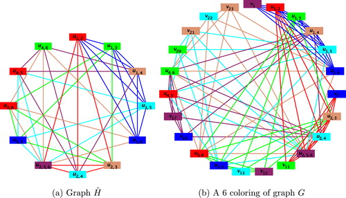
Let $G$ be the graph shown in Fig. 14a.

Let $V\left(A_1\right)=\{v_1,v_2,v_3,v_4,v_5,v_6\}$, $V\left(A_2\right)=\{v_2,v_7,v_8,v_9,v_{10},v_{11}\}$,

$V\left(A_3\right)=\{v_3,v_8,v_{12},v_{13},v_{14},v_{15}\}$, $V\left(A_4\right)=\{v_4,v_9,v_{16},v_{17},v_{18},v_{20},v_{21}\}$,

$V\left(A_5\right)=\{v_5,v_{10},v_{14},v_{18},v_{20},v_{21}\}$, $V\left(A_6\right)=\{v_6,v_{10},v_{15},v_{19},v_{22},v_{23}\}$.

Relabel the vertices of clique degree greater than one in $G$ by $u_A$ where $A=\{i:v\in A_i\text{for}1\le i\le 6\}$. The labeled graph is shown in Fig. 14b. Fig. 15 is the graph $\hat{H}$, where $\hat{H}$ is obtained by removing the vertices of clique degree 1 from $G$.

Let $X=\{b_{ij}:A_i\cap A_j=0̸\}=\left\{b_{3,4}\right\}$, $$X_1=\{v\in G:d^K\left(v\right)=1\}=\{v_1,v_7,v_{11},v_{12},v_{13},v_{16},v_{17},v_{20},v_{21},v_{22},v_{23}\},$$ $$X_2=\{v\in G:d^K\left(v\right)=2\}=\{v_2,v_3,v_4,v_5,v_6,v_8,v_9,v_{14},v_{15},v_{18},v_{19}\}=\{u_{1,2},u_{1,3},u_{1,4},u_{1,5},u_{1,6},u_{2,3},u_{2,4},u_{3,5},u_{3,6},u_{4,5},u_{4,6}\},$$ and $X_3=\{v\in G:d^K\left(v\right)=3\}=\left\{v_{10}\right\}=\left\{u_{2,5,6}\right\}$.

Let 1, 2, $\dots$, 6 be the six colors and $C=\left(\begin{array}{cccccc}\hfill 6\hfill & \hfill 1\hfill & \hfill 2\hfill & \hfill 3\hfill & \hfill 4\hfill & \hfill 5\hfill \\ \hfill 1\hfill & \hfill 3\hfill & \hfill 5\hfill & \hfill 6\hfill & \hfill 2\hfill & \hfill 4\hfill \\ \hfill 2\hfill & \hfill 5\hfill & \hfill 4\hfill & \hfill 1\hfill & \hfill 6\hfill & \hfill 3\hfill \\ \hfill 3\hfill & \hfill 6\hfill & \hfill 1\hfill & \hfill 4\hfill & \hfill 5\hfill & \hfill 2\hfill \\ \hfill 4\hfill & \hfill 2\hfill & \hfill 6\hfill & \hfill 5\hfill & \hfill 3\hfill & \hfill 1\hfill \\ \hfill 5\hfill & \hfill 4\hfill & \hfill 3\hfill & \hfill 2\hfill & \hfill 1\hfill & \hfill 6\hfill \end{array}\right)$ be the color matrix (as well as symmetric latin square) of order 6 × 6.

Consider the sets $T=X_3=\left\{u_{2,5,6}\right\}$,

$T^{\prime \prime }=X_2=\{u_{1,2},u_{1,3},u_{1,4},u_{1,5},u_{1,6},u_{2,3},u_{2,4},u_{3,5},u_{3,6},u_{4,5},u_{4,6}\}$, $P=0̸$ and $P^{\prime \prime }=0̸$. Then by applying the aforementioned method we get a new color matrix $C_1$ by putting $c_{i,j}=0$, $c_{j,i}=0$ for every $b_{i,j}$ in $X$ and $c_{i,i}=0$ for each $i=1,2,\dots ,6$ and go to Step 1. $$C_1=\left(\begin{array}{cccccc}\hfill 0\hfill & \hfill 1\hfill & \hfill 2\hfill & \hfill 3\hfill & \hfill 4\hfill & \hfill 5\hfill \\ \hfill 1\hfill & \hfill 0\hfill & \hfill 5\hfill & \hfill 6\hfill & \hfill 2\hfill & \hfill 4\hfill \\ \hfill 2\hfill & \hfill 5\hfill & \hfill 0\hfill & \hfill 0\hfill & \hfill 6\hfill & \hfill 3\hfill \\ \hfill 3\hfill & \hfill 6\hfill & \hfill 0\hfill & \hfill 0\hfill & \hfill 5\hfill & \hfill 2\hfill \\ \hfill 4\hfill & \hfill 2\hfill & \hfill 6\hfill & \hfill 5\hfill & \hfill 0\hfill & \hfill 1\hfill \\ \hfill 5\hfill & \hfill 4\hfill & \hfill 3\hfill & \hfill 2\hfill & \hfill 1\hfill & \hfill 0\hfill \end{array}\right)$$

Step 1: Since $T\ne 0̸$, choose the vertex $u_{2,5,6}$ from $T$. Let $T^{\prime }=\{b_{2,5},b_{2,6},b_{5,6}\}$ and $P^{\prime }=0̸$, then $T_1^{\prime }=0̸$ and $T_2^{\prime }=T^{\prime }$. Since $T_1^{\prime }=0̸$, choose the vertex $b_{5,6}$ from $T_2^{\prime }$, add it to $P^{\prime }$ and remove it from $T^{\prime }$. Then $T^{\prime }=\{b_{2,5},b_{2,6}\}$ and $P^{\prime }=\left\{b_{5,6}\right\}$. Go to step 2.

Step 2: Since $T_2^{\prime }\ne 0̸$, go to step 3.

Step 3: Since $T^{\prime }\ne 0̸$ and $T^{\prime }\cap T_1^{\prime }=0̸$, choose the vertex $b_{2,5}$ from $T^{\prime }\cap T_2^{\prime }$ and go to step 4.

Step 4: Since $c\left(b_{2,5}\right)=2$, $c\left(b_{5,6}\right)=1$ and $c\left(b_{2,5}\right)\ne c\left(b_{5,6}\right)$, interchange 2, 1 in the matrix $C_1$ except the color of $b_{5,6}$. Add the vertex $b_{2,5}$ to $P^{\prime }$ and remove it from $T^{\prime }$. Then $$C_2=\left(\begin{array}{cccccc}\hfill 0\hfill & \hfill 2\hfill & \hfill 1\hfill & \hfill 3\hfill & \hfill 4\hfill & \hfill 5\hfill \\ \hfill 2\hfill & \hfill 0\hfill & \hfill 5\hfill & \hfill 6\hfill & \hfill 1\hfill & \hfill 4\hfill \\ \hfill 1\hfill & \hfill 5\hfill & \hfill 0\hfill & \hfill 0\hfill & \hfill 6\hfill & \hfill 3\hfill \\ \hfill 3\hfill & \hfill 6\hfill & \hfill 0\hfill & \hfill 0\hfill & \hfill 5\hfill & \hfill 2\hfill \\ \hfill 4\hfill & \hfill 1\hfill & \hfill 6\hfill & \hfill 5\hfill & \hfill 0\hfill & \hfill 1\hfill \\ \hfill 5\hfill & \hfill 4\hfill & \hfill 3\hfill & \hfill 2\hfill & \hfill 1\hfill & \hfill 0\hfill \end{array}\right),$$

$T^{\prime }=\left\{b_{2,6}\right\}$ and $P^{\prime }=\{b_{2,5},b_{5,6}\}$. Go to step 3.

Step 3: Since $T^{\prime }\ne 0̸$ and $T^{\prime }\cap T_1^{\prime }=0̸$, choose the vertex $b_{2,6}$ from $T^{\prime }\cap T_2^{\prime }$ and go to step 4.

Step 4: Since $c\left(b_{2,6}\right)=4$, $c\left(b_{5,6}\right)=1$ and $c\left(b_{2,6}\right)\ne c\left(b_{5,6}\right)$, interchange 4, 1 in the matrix $C_2$ except the color of $b_{2,5},b_{5,6}$. Add the vertex $b_{2,6}$ to $P^{\prime }$ and remove it from $T^{\prime }$. Then $$C_3=\left(\begin{array}{cccccc}\hfill 0\hfill & \hfill 2\hfill & \hfill 4\hfill & \hfill 3\hfill & \hfill 1\hfill & \hfill 5\hfill \\ \hfill 2\hfill & \hfill 0\hfill & \hfill 5\hfill & \hfill 6\hfill & \hfill 1\hfill & \hfill 1\hfill \\ \hfill 4\hfill & \hfill 5\hfill & \hfill 0\hfill & \hfill 0\hfill & \hfill 6\hfill & \hfill 3\hfill \\ \hfill 3\hfill & \hfill 6\hfill & \hfill 0\hfill & \hfill 0\hfill & \hfill 5\hfill & \hfill 2\hfill \\ \hfill 1\hfill & \hfill 1\hfill & \hfill 6\hfill & \hfill 5\hfill & \hfill 0\hfill & \hfill 1\hfill \\ \hfill 5\hfill & \hfill 1\hfill & \hfill 3\hfill & \hfill 2\hfill & \hfill 1\hfill & \hfill 0\hfill \end{array}\right),$$

$T^{\prime }=0̸$ and $P^{\prime }=\{b_{2,5},b_{2,6},b_{5,6}\}$. Go to step 3.

Step 3: Since $T^{\prime }=0̸$, add the vertex $u_{2,5,6}$ to $P$ and remove it from $T$, then $T=0̸$ and $P=\left\{u_{2,5,6}\right\}$. Go to step 1.

Step 1: Since $T=0̸$ consider $C_m=C_3$, go to step 5.

Step 5: Since $T^{\prime \prime }\ne 0̸$, choose the vertex $u_{1,2}$ from $T^{\prime \prime }$. Go to step 6.

Step 6: Since $c_{1,2}=2$ appears exactly once in both 1st row and 2nd column of the color matrix $C_m$. Add the vertex $u_{1,2}$ to $P^{\prime \prime }$ and remove it from $T^{\prime \prime }$. Then $T^{\prime \prime }=\{u_{1,3},u_{1,4},u_{1,5},u_{1,6},u_{2,3},u_{2,4},u_{3,5},u_{3,6},u_{4,5},u_{4,6}\}$ and $P^{\prime \prime }=\left\{u_{1,2}\right\}$. Go to Step 5.

Step 5: Since $T^{\prime \prime }\ne 0̸$, choose the vertex $u_{1,3}$ from $T^{\prime \prime }$. Go to step 6.

Step 6: Since $c_{1,3}=4$ appears exactly once in both 1st row and 3rd column of the color matrix $C_m$. Add the vertex $u_{1,3}$ to $P^{\prime \prime }$ and remove it from $T^{\prime \prime }$. Then $T^{\prime \prime }=\{u_{1,4},u_{1,5},u_{1,6},u_{2,3},u_{2,4},u_{3,5},u_{3,6},u_{4,5},u_{4,6}\}$ and $P^{\prime \prime }=\{u_{1,2},u_{1,3}\}$. Go to Step 5.

Step 5: Since $T^{\prime \prime }\ne 0̸$, choose the vertex $u_{1,4}$ from $T^{\prime \prime }$. Go to step 6.

Step 6: Since $c_{1,4}=3$ appears exactly once in both 1st row and 4th column of the color matrix $C_m$. Add the vertex $u_{1,4}$ to $P^{\prime \prime }$ and remove it from $T^{\prime \prime }$. Then $T^{\prime \prime }=\{u_{1,5},u_{1,6},u_{2,3},u_{2,4},u_{3,5},u_{3,6},u_{4,5},u_{4,6}\}$ and $P^{\prime \prime }=\{u_{1,2},u_{1,3},u_{1,4}\}$. Go to Step 5.

Step 5: Since $T^{\prime \prime }\ne 0̸$, choose the vertex $u_{1,5}$ from $T^{\prime \prime }$. Go to step 6.

Step 6: Since $c_{1,5}=1$ and it appears more than once in the 5th column of the color matrix $C_m$. Let $A=\{c_{1,j}:c_{1,j}\ne 0;1\le j\le 6\}=\{1,2,3,4,5\}$, $B=\{c_{i,5}:c_{i,5}\ne 0;1\le i\le 6\}=\{1,5,6\}$, then $A\cup B$ = {1, 2, 3, 4, 5, 6} and $\{1,2,3,4,5,6\}\setminus A\cup B=0̸$.

It cannot be go further.

In the illustration of Example 4.3, if we choose the color matrix (symmetric latin square) given below, then exists an $n$-coloring of $G$.

Let $C^{\prime }=\left(\begin{array}{cccccc}\hfill 1\hfill & \hfill 2\hfill & \hfill 3\hfill & \hfill 4\hfill & \hfill 5\hfill & \hfill 6\hfill \\ \hfill 2\hfill & \hfill 3\hfill & \hfill 4\hfill & \hfill 5\hfill & \hfill 6\hfill & \hfill 1\hfill \\ \hfill 3\hfill & \hfill 4\hfill & \hfill 5\hfill & \hfill 6\hfill & \hfill 1\hfill & \hfill 2\hfill \\ \hfill 4\hfill & \hfill 5\hfill & \hfill 6\hfill & \hfill 1\hfill & \hfill 2\hfill & \hfill 3\hfill \\ \hfill 5\hfill & \hfill 6\hfill & \hfill 1\hfill & \hfill 2\hfill & \hfill 3\hfill & \hfill 4\hfill \\ \hfill 6\hfill & \hfill 1\hfill & \hfill 2\hfill & \hfill 3\hfill & \hfill 4\hfill & \hfill 5\hfill \end{array}\right)$.

Applying the method in Example 4.3, we get $$C_M^{\prime }=\left(\begin{array}{cccccc}\hfill 0\hfill & \hfill 2\hfill & \hfill 3\hfill & \hfill 6\hfill & \hfill 5\hfill & \hfill 1\hfill \\ \hfill 2\hfill & \hfill 0\hfill & \hfill 6\hfill & \hfill 5\hfill & \hfill 4\hfill & \hfill 4\hfill \\ \hfill 3\hfill & \hfill 6\hfill & \hfill 0\hfill & \hfill 0\hfill & \hfill 1\hfill & \hfill 2\hfill \\ \hfill 6\hfill & \hfill 5\hfill & \hfill 0\hfill & \hfill 0\hfill & \hfill 2\hfill & \hfill 3\hfill \\ \hfill 5\hfill & \hfill 4\hfill & \hfill 1\hfill & \hfill 2\hfill & \hfill 0\hfill & \hfill 4\hfill \\ \hfill 1\hfill & \hfill 4\hfill & \hfill 2\hfill & \hfill 3\hfill & \hfill 4\hfill & \hfill 0\hfill \end{array}\right).$$

Color the vertex $v$ by the $(i,j)$th entry $c_{i,j}$ of the matrix $C_M^{\prime }$, whenever $A_i\cap A_j\ne 0̸$ (see Fig. 16a), where the numbers 1, 2, 3, 4, 5, 6 correspond to the colors Blue, Red, Green, Maroon, Tan, Cyan respectively. Extend the coloring of $\hat{H}$ to $G$ by assigning the remaining colors which are not used for $A_i$ from the set of $6$-colors to the vertices of clique degree one in each $A_i$, $1\le i\le 6$. The colored graph $G$ is shown in Fig. 16b.

Remark 4.4

From the above example, one can see that the method will work for some symmetric latin squares and will not work for some other, for the graphs having more than $\frac{n}{2}$ vertices of clique degree greater than one in some $A_i$ ($1\le i\le n$) in $G$.

Acknowledgment

We thank Dr. Vance Faber, Center for Computing Sciences, Bowie, MD, USA for his valuable suggestions during this research work.

References

- BergeClaude, On two conjectures to generalize Vizing’s theorem Matematiche (Catania) 45 1 1990 15–23 (1991)Graphs, designs and combinatorial geometries (Catania, 1989)
- ErdősPAUL, Problems and results in graph theory and combinatorial analysis Proc. British Combinatorial Conj., 5th1975 169–192
- ErdősPál, On the combinatorial problems which i would most like to see solved Combinatorica 1 1 1981 25–42
- JensenTommy RToftBjarne, Graph Coloring Problems, Vol. 392011John Wiley & Sons
- ChangWilliam I.LawlerEugene L., Edge coloring of hypergraphs and a conjecture of Erdös, Faber, Lovász Combinatorica 8 3 1988 293–295
- KahnJeff, Coloring nearly-disjoint hypergraphs with n+o(n) colors J. Combin. Theory Ser. A 59 1 1992 31–39
- JacksonBillSethuramanG.WhiteheadCarol, A note on the Erdős-Farber-Lovász conjecture Discrete Math. 307 7–8 2007 911–915
- PaulVijiGerminaK.A., On edge coloring of hypergraphs and Erdös-Faber-Lovász conjecture Discrete Math. Algorithms Appl. 4 1 2012 12500035
- Sánchez-ArroyoAbdón, The Erdős-Faber-Lovász conjecture for dense hypergraphs Discrete Math. 308 5–6 2008 991–992
- DezaMErdösPFranklP, Intersection properties of systems of finite sets Proc. Lond. Math. Soc. 3 2 1978 369–384
- MitchemJohnSchmidtRandolph L., On the Erdős-Faber-Lovász conjecture Ars Combin. 972010 497–505
- HaddadLucienTardifClaude, A clone-theoretic formulation of the Erdös-Faber-Lovász conjecture Discuss. Math. Graph Theory 24 3 2004 545–549
- KunduSukhamaySampathkumarEShearerJamesSturtevantDean, Reconstruction of a pair of graphs from their concatenations SIAM J. Algebr. Discrete Methods 1 2 1980 228–231
- LaywineCharles FMullenGary L, Discrete Mathematics using Latin Squares, Vol. 171998Wiley New York
- YeXiaoruiXuYunqing, On the number of symmetric latin squares Computer Science and Service System (CSSS), 2011 International Conference on2011IEEE2366–2369
- BryantDarrynRodgerCA, On the completion of latin rectangles to symmetric latin squares J. Aust. Math. Soc. 76 1 2004 109–124