A combinatorial interpretation of the bijection of Goulden and Yong

Abstract

We define a dual of a graph, generalizing the definition of Goulden et al. (2002), which only applies to trees; then we reprove their main result using our new definition. We in fact give two characterizations of the dual: a graph-theoretic one and an algebraic one, showing that they are in fact the same, and are also the same (on trees) as the topological dual developed by Goulden and Yong. Goulden and Yong use their dual to define a bijection between the vertex labeled trees and the factorizations of the permutation $(n,\dots ,1)$ into $n-1$ transpositions, showing that their bijection has a particular structural property. We give a combinatorial, non-topological, proof of their result, using our dual.

Keywords:

• Factorizations
• Transpositions
• Dual
• Bijection

1 Introduction

The basic objects we investigate are factorizations of permutations into transpositions. By ${\mathbf{S}}_n$ we mean the symmetric group on the set $\left[n\right]=\{1,2,\dots ,n\}$; for us, all multiplication is from left to right. To refer to “factorizations” precisely we introduce the notion of a transposition sequence: a transposition sequence (over ${\mathbf{S}}_n$) is a sequence of transpositions in ${\mathbf{S}}_n$.

Example 1.1

The sequence $〈(3,4),(1,3),(1,2),(3,4),(2,3)〉$ is a transposition sequence over ${\mathbf{S}}_4$.

Dénes [1] showed that there are exactly $n^{n-2}$ factorizations of $(n,\dots ,2,1)$ into $n-1$ transpositions. Since it is well-known that there are also $n^{n-2}$ vertex labeled trees on $n$ vertices, Dénes suggested the project of finding interesting bijections between these factorizations and these trees. While interesting in its own right, the project posed by Dénes is further motivated by fitting it into a broader context suggested by [2] and [3]. A factorization of $(n,\dots ,2,1)$ into $n-1$ transpositions is in fact what is called a minimal transitive factorization; any permutation of ${\mathbf{S}}_n$ can be factored into its minimal transitive factorizations. Minimal transitive factorizations are of interest because of their connection to topology (for example, see [4] and [5]); this work also has connections to more recent work in topology, for example [6].

Definition 1.2

–	Let ${\mathcal{F}}^{(n\dots 1)}$ be the set of length $n-1$ transposition sequences over ${\mathbf{S}}_n$, with product $(n,\dots ,2,1)$.
–	Let ${\mathcal{T}}_n$ be the set of trees on $n$ vertices, so that each vertex gets a distinct label from the set $\left[n\right]$.

Using this terminology, Dénes’ challenge is to find bijections between ${\mathcal{F}}^{(n\dots 1)}$ and ${\mathcal{T}}_n$. Moszkowski [7] found a bijection in 1989; then in 1993 Goulden and Pepper [8] found a different bijection. However, arguably the nicest bijection is developed in 2002 by Goulden and Yong [3]; in this bijection, various structural properties are preserved. An example of a structural property is this: if we consider a factorization and the tree it is mapped to, the number of transpositions which are consecutive pairs (i.e. $(n,1)$ or of the form $(x,x+1)$) in the factorization is the same as the number of leaves in the tree. Further nice properties of this bijection, including enumerative consequences, are discussed in [3]. Essential in the bijection of [3] is their definition of the dual of a tree, defined topologically; a similar dual was defined in 1999 by Herando Martín [9]. The main point of our work is an alternative definition of the dual and an alternative combinatorial proof of the Goulden and Yong result, which avoids topology; in fact we will give two equivalent definitions of our dual, which, on trees, are equivalent to the dual of [3].

In Section 2 we give an algebraic definition of the dual. Section 3 describes a graph-theoretic interpretation of transposition sequences. In Section 4, in Theorem 4.7, we give one of our main results, an alternate proof of the main result from [3] using our dual. Section 5 gives an equivalent graph-theoretic definition of the dual. In Section 6 we prove that our dual (when restricted to trees) is in fact the same as the topological dual of [3]. In Section 7 we investigate a technical property related to the graph-theoretic dual. Our dual is interesting because it applies to all finite graphs, coincides with the dual of [3] for trees, and allows us to give an alternate combinatorial proof of the main result from [3].

2 Algebraic dual

For permutations $\alpha$ and $\beta$, let ${\mathsf{\beta }}^{\mathsf{\alpha }}$ be the conjugate $\mathsf{\alpha }\mathsf{\beta }{\mathsf{\alpha }}^{-1}$.

Definition 2.1

The Algebraic Dual of $〈{\mathsf{s}}_{\mathsf{1}},\dots ,{\mathsf{s}}_{\mathsf{m}}〉$ is $〈{\mathsf{s}}_{\mathsf{1}},{{\mathsf{s}}_{\mathsf{2}}}^{{\mathsf{s}}_{\mathsf{1}}},{{\mathsf{s}}_{\mathsf{3}}}^{{\mathsf{s}}_{\mathsf{1}}{\mathsf{s}}_{\mathsf{2}}},\dots ,{{\mathsf{s}}_{\mathsf{m}}}^{{\mathsf{s}}_{\mathsf{1}}\cdots {\mathsf{s}}_{\mathsf{m}-\mathsf{1}}}〉$.

We will often denote the Algebraic Dual of a transposition sequence $\mathbf{s}$ by ${\mathbf{s}}^{\prime }$.

Example 2.2

We calculate the Algebraic Dual of $\mathbf{s}=〈(3,4),(1,3),(1,2),(3,4),(2,3)〉$, the transposition sequence of Example 1.1. $${{\mathsf{s}}_{\mathsf{2}}}^{{\mathsf{s}}_{\mathsf{1}}}={(1,3)}^{(3,4)}=(1,4)\text{and}{{\mathsf{s}}_{\mathsf{3}}}^{{\mathsf{s}}_{\mathsf{1}}{\mathsf{s}}_{\mathsf{2}}}={(1,2)}^{(3,4)(1,3)}=(2,4)$$Continuing, we see that the Algebraic Dual ${\mathbf{s}}^{\prime }$ is $〈(3,4),(1,4),(2,4),(1,3),(3,4)〉$.

We now prove three important properties of the Algebraic Dual, in Lemmas 2.3, 2.4, and 2.5.

Lemma 2.3

For any transposition sequence $〈{\mathsf{s}}_{\mathsf{1}},\dots ,{\mathsf{s}}_{\mathsf{m}}〉$ and its Algebraic Dual $〈{\mathsf{s}}_{\mathsf{1}}^{\prime },\dots ,{\mathsf{s}}_{\mathsf{m}}^{\prime }〉$, the product ${\mathsf{s}}_{\mathsf{1}}\cdots {\mathsf{s}}_{\mathsf{m}}$ is the inverse of the product ${\mathsf{s}}_{\mathsf{1}}^{\prime }\cdots {\mathsf{s}}_{\mathsf{m}}^{\prime }$.

Proof

Basically we multiply out the transpositions and cancel appropriately, as shown in the following calculation. $${\mathsf{s}}_{\mathsf{1}}^{\prime }\cdots {\mathsf{s}}_{\mathsf{m}}^{\prime }={\mathsf{s}}_{\mathsf{1}}\cdot {{\mathsf{s}}_{\mathsf{2}}}^{{\mathsf{s}}_{\mathsf{1}}}\cdot {{\mathsf{s}}_{\mathsf{3}}}^{{\mathsf{s}}_{\mathsf{1}}\cdot {\mathsf{s}}_{\mathsf{2}}}\cdots {{\mathsf{s}}_{\mathsf{m}}}^{{\mathsf{s}}_{\mathsf{1}}\cdots {\mathsf{s}}_{\mathsf{m-1}}}={\mathsf{s}}_{\mathsf{1}}\cdot \left({\mathsf{s}}_{\mathsf{1}}\cdot {\mathsf{s}}_{\mathsf{2}}\cdot {\mathsf{s}}_{\mathsf{1}}\right)\cdot \left({\mathsf{s}}_{\mathsf{1}}\cdot {\mathsf{s}}_{\mathsf{2}}\cdot {\mathsf{s}}_{\mathsf{3}}\cdot {\mathsf{s}}_{\mathsf{2}}\cdot {\mathsf{s}}_{\mathsf{1}}\right)\cdots ={\mathsf{s}}_{\mathsf{m}}\cdots {\mathsf{s}}_{\mathsf{1}}\square$$

Lemma 2.4

For any transposition sequence $\mathsf{s}$ we have ${\mathsf{s}}^{\prime \prime }=\mathsf{s}$.

Proof

Suppose $\mathsf{s}=〈{\mathsf{s}}_{\mathsf{1}},\dots ,{\mathsf{s}}_{\mathsf{m}}〉$ and ${\mathsf{s}}^{\prime \prime }=〈{\mathsf{s}}_{\mathsf{1}}^{\prime \prime },\dots ,{\mathsf{s}}_{\mathsf{m}}^{\prime \prime }〉$. Consider any $k=1,\dots ,m$, and we show that ${\mathsf{s}}_{\mathsf{k}}^{\prime \prime }={\mathsf{s}}_{\mathsf{k}}$. $${\mathsf{s}}_{\mathsf{k}}^{\prime \prime }={\left({{\mathsf{s}}_{\mathsf{k}}}^{{\mathsf{s}}_{\mathsf{1}}\cdots {\mathsf{s}}_{\mathsf{k-1}}}\right)}^{{\mathsf{s}}_{\mathsf{1}}\cdot {{\mathsf{s}}_{\mathsf{2}}}^{{\mathsf{s}}_{\mathsf{1}}}\cdots {{\mathsf{s}}_{\mathsf{k-1}}}^{{\mathsf{s}}_{\mathsf{1}}\cdots {\mathsf{s}}_{\mathsf{k-2}}}}\text{applying the definition of Algebraic}\text{Dual twice}={\left({{\mathsf{s}}_{\mathsf{k}}}^{{\mathsf{s}}_{\mathsf{1}}\cdots {\mathsf{s}}_{\mathsf{k-1}}}\right)}^{{\mathsf{s}}_{\mathsf{k-1}}\cdots {\mathsf{s}}_{\mathsf{1}}}\text{by Lemma}\text{2.3}=({\mathsf{s}}_{\mathsf{k-1}}\cdots {\mathsf{s}}_{\mathsf{1}})\cdot ({\mathsf{s}}_{\mathsf{1}}\cdots {\mathsf{s}}_{\mathsf{k-1}}\cdot {\mathsf{s}}_{\mathsf{k}}\cdot {\mathsf{s}}_{\mathsf{k-1}}\cdots {\mathsf{s}}_{\mathsf{1}})\cdot ({\mathsf{s}}_{\mathsf{1}}\cdots {\mathsf{s}}_{\mathsf{k-1}})={\mathsf{s}}_{\mathsf{k}}\square$$

Let ${〈{\mathsf{s}}_{\mathsf{1}},\dots ,{\mathsf{s}}_{\mathsf{k}}〉}^{\mathsf{t}}$ be $〈{{\mathsf{s}}_{\mathsf{1}}}^{\mathsf{t}},\dots ,{{\mathsf{s}}_{\mathsf{k}}}^{\mathsf{t}}〉$, and let $〈{\mathsf{s}}_{\mathsf{1}}〉〈{\mathsf{s}}_{\mathsf{2}},\dots ,{\mathsf{s}}_{\mathsf{m}}〉$ be $〈{\mathsf{s}}_{\mathsf{1}},{\mathsf{s}}_{\mathsf{2}},\dots ,{\mathsf{s}}_{\mathsf{m}}〉$.

Lemma 2.5

${\left(〈{\mathsf{s}}_{\mathsf{1}}〉{〈{\mathsf{s}}_{\mathsf{2}},\dots ,{\mathsf{s}}_{\mathsf{m}}〉}^{\prime }\right)}^{{\mathsf{s}}_{\mathsf{1}}}={〈{\mathsf{s}}_{\mathsf{1}},\dots ,{\mathsf{s}}_{\mathsf{m}}〉}^{\prime }$

Proof

Using the definition of the Algebraic Dual and properties of conjugation, we can make the following calculation. $${\left(〈{\mathsf{s}}_{\mathsf{1}}〉{〈{\mathsf{s}}_{\mathsf{2}},\dots ,{\mathsf{s}}_{\mathsf{m}}〉}^{\prime }\right)}^{{\mathsf{s}}_{\mathsf{1}}}={〈{\mathsf{s}}_{\mathsf{1}},{\mathsf{s}}_{\mathsf{2}},{{\mathsf{s}}_{\mathsf{3}}}^{{\mathsf{s}}_{\mathsf{2}}},\dots ,{{\mathsf{s}}_{\mathsf{m}}}^{{\mathsf{s}}_{\mathsf{2}}\cdots {\mathsf{s}}_{\mathsf{m-1}}}〉}^{{\mathsf{s}}_{\mathsf{1}}}=〈{{\mathsf{s}}_{\mathsf{1}}}^{{\mathsf{s}}_{\mathsf{1}}},{{\mathsf{s}}_{\mathsf{2}}}^{{\mathsf{s}}_{\mathsf{1}}},{\left({{\mathsf{s}}_{\mathsf{3}}}^{{\mathsf{s}}_{\mathsf{2}}}\right)}^{{\mathsf{s}}_{\mathsf{1}}},\dots ,{\left({{\mathsf{s}}_{\mathsf{m}}}^{{\mathsf{s}}_{\mathsf{2}}\cdots {\mathsf{s}}_{\mathsf{m-1}}}\right)}^{{\mathsf{s}}_{\mathsf{1}}}〉=〈{\mathsf{s}}_{\mathsf{1}},{{\mathsf{s}}_{\mathsf{2}}}^{{\mathsf{s}}_{\mathsf{1}}}{{\mathsf{s}}_{\mathsf{3}}}^{{\mathsf{s}}_{\mathsf{1}}\cdot {\mathsf{s}}_{\mathsf{2}}},\dots ,{{\mathsf{s}}_{\mathsf{m}}}^{{\mathsf{s}}_{\mathsf{1}}\cdot {\mathsf{s}}_{\mathsf{2}}\cdots {\mathsf{s}}_{\mathsf{m-1}}}〉={〈{\mathsf{s}}_{\mathsf{1}},\dots ,{\mathsf{s}}_{\mathsf{m}}〉}^{\prime }\square$$

Note that Lemmas 2.3 and 2.4 would hold if we defined the Algebraic Dual of a transposition sequence $〈{\mathsf{s}}_{\mathsf{1}},\dots ,{\mathsf{s}}_{\mathsf{m}}〉$ to simply be its reverse $〈{\mathsf{s}}_{\mathsf{m}},\dots ,{\mathsf{s}}_{\mathsf{1}}〉$, but Lemma 2.5 would fail; Lemma 2.5 will be crucial to later developments.

The next lemma gives an interesting alternative way to view the Algebraic Dual.

Lemma 2.6

For a transposition sequence $〈{\mathsf{s}}_{\mathsf{1}},\dots ,{\mathsf{s}}_{\mathsf{m}}〉$ and its Algebraic Dual $〈{\mathsf{s}}_{\mathsf{1}}^{\prime },\dots ,{\mathsf{s}}_{\mathsf{m}}^{\prime }〉$, $${\mathsf{s}}_{\mathsf{k}}^{\prime }=({\alpha }^{-1}\left(x\right),{\alpha }^{-1}\left(y\right)),$$where ${\mathsf{s}}_{\mathsf{k}}=(x,y)$ and $\alpha ={\mathsf{s}}_{\mathsf{1}}\cdots {\mathsf{s}}_{\mathsf{k-1}}$.

Proof

$${{\mathsf{s}}_{\mathsf{k}}}^{\prime }={{\mathsf{s}}_{\mathsf{k}}}^{{\mathsf{s}}_{\mathsf{1}}\cdots {\mathsf{s}}_{\mathsf{k-1}}}={{\mathsf{s}}_{\mathsf{k}}}^{\alpha }=\alpha \cdot (x,y)\cdot {\alpha }^{-1}=({\alpha }^{-1}\left(x\right),{\alpha }^{-1}\left(y\right))$$

We can see that the last equality is true by viewing $\alpha \cdot (x,y)\cdot {\alpha }^{-1}$ as first mapping ${\alpha }^{-1}\left(x\right)$ to $x$, then $x$ to $y$, then $y$ to ${\alpha }^{-1}\left(y\right)$. Similarly ${\alpha }^{-1}\left(y\right)$ is mapped to ${\alpha }^{-1}\left(x\right)$, and furthermore, any other element (besides ${\alpha }^{-1}\left(x\right)$ and ${\alpha }^{-1}\left(y\right)$) is mapped to itself.□

This lemma provides a visual way to understand the Algebraic Dual, which we illustrate via an example. Consider Example 2.2 where we have the transposition sequence $\mathbf{s}$ and its Algebraic Dual ${\mathbf{s}}^{\prime }$. The product of the transpositions in $\mathbf{s}$ yields the permutation $(4,3,2,1)$; this result can also be achieved by starting with $\left(\genfrac{}{}{0ex}{}{1,2,3,4}{1,2,3,4}\right)$, the identity permutation written in inline notation, and successively swapping the bottom numbers according to $\mathbf{s}$, i.e. to get $\left(\genfrac{}{}{0ex}{}{1,2,3,4}{1,2,4,3}\right)$, then $\left(\genfrac{}{}{0ex}{}{1,2,3,4}{3,2,4,1}\right)$, and so on till we get $\left(\genfrac{}{}{0ex}{}{1,2,3,4}{4,1,2,3}\right)$. Lemma 2.6 tells us that if we want to get the same result by swapping the top elements of the inline notation, then the Algebraic Dual provides the required swaps; for example, if we use ${\mathbf{s}}^{\prime }$ from Example 2.2, then we start with the identity $\left(\genfrac{}{}{0ex}{}{1,2,3,4}{1,2,3,4}\right)$, then get $\left(\genfrac{}{}{0ex}{}{1,2,4,3}{1,2,3,4}\right)$, then get $\left(\genfrac{}{}{0ex}{}{4,2,1,3}{1,2,3,4}\right)$, and continue till we get $\left(\genfrac{}{}{0ex}{}{2,3,4,1}{1,2,3,4}\right)$, which is the permutation $(4,3,2,1)$.

3 Graph interpretation

We describe a standard way that transposition sequences are viewed as labeled graphs, using this interpretation in Section 4 in order to define the bijection, and in Section 5 in order to define the Graph Dual. For us, a graph will always mean a finite, loop-less graph, with multi-edges allowed. A labeled graph is a graph whose $n$ vertices are labeled by $\left[n\right]$ (each vertex receiving a distinct label), and whose $m$ edges are labeled by $\left[m\right]$ (each edge receiving a distinct label). As is commonly done (for example, in [3]) we view $〈{\mathsf{s}}_{\mathsf{1}},\dots ,{\mathsf{s}}_{\mathsf{m}}〉$, a transposition sequence over ${\mathbf{S}}_n$, as a labeled graph with vertex set $\left[n\right]$, with $m$ edges: For each transposition ${\mathsf{s}}_{\mathsf{i}}=(x_i,y_i)$ we create a corresponding edge between $x_i$ and $y_i$, labeled by $i$. Fig. 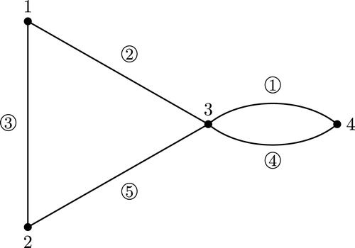1 displays the transposition sequence of Example 1.1 as a graph.

Fig. 1 The transposition sequence from Example 1.1 written as a labeled graph.

Following usual definitions, we define a trail to be a non-empty sequence $〈v_1,e_1,v_2,e_2,\dots ,v_{k-1},e_{k-1},v_k〉$ such that each $v_i$ is a vertex, each $e_i=\{v_i,v_{i+1}\}$ is an edge, and no edge is repeated (vertices may be repeated). Notice that trails are ordered with a start vertex of $v_1$ and end vertex of $v_k$. For us, the trails of fundamental interest are given in the next definition.

Definition 3.1

Consider a labeled graph and any vertex $u$. The Minimal Increasing Greedy Trail (MIGT) starting at $u$ is the trail $〈v_1,e_1,v_2,e_2,\dots ,v_{k-1},e_{k-1},v_k〉$ such that $v_1$ is $u$, and each edge $e_j$ is the edge incident to $v_j$ with the smallest label which is larger than all the labels on edges $e_i$ ($i<j$) which are incident to $v_j$. The trail ends when there is no such edge $e_j$. This (unique) trail is referred to by ${\mathsf{T}}_u$.

Example 3.2

Referring to the graph in Fig. 1, ${\mathsf{T}}_3$ is the following trail: $〈3,\overline{1},4,\overline{4},3,\overline{5},2〉$, where we write $\overline{e}$ to refer to the unique edge with label $e$.

4 Alternate proof for Goulden/Yong bijection

In this section we use our framework to describe a bijection between the vertex labeled trees and the factorizations of $(n,\dots ,2,1)$ into $n-1$ transpositions. Following [3] we define the bijection as the composition of a relabeling function with our dual. We will show, in Section 6, that our dual is the same as that of [3], so in fact, the bijection we are describing is the same as that of [3]. We give an alternate proof, using our dual, that the bijection possesses the structural properties described in [3].

4.1 The bijection

For the purposes of this paper, we define a Minimal Transitive Factorization over ${\mathbf{S}}_n$ to be a transposition sequence of length $n-1$ whose product is a single cycle involving all the elements of $\left[n\right]$. Immediate from Dénes [1] we have the following theorem; the coherence of the subsequent definitions and discussion depends on this fact.

Theorem 4.1

[1] A transposition sequence is a Minimal Transitive Factorization over${\mathbf{S}}_n$ if and only if it is a tree whose vertices are $\left[n\right]$

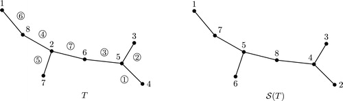
In Definition 1.2 we defined ${\mathcal{F}}^{(n\dots 1)}$; we now define ${\mathcal{F}}^{(1\dots n)}$ to be the set of length $n-1$ transposition sequences over ${\mathbf{S}}_n$ with product $(1,2,\dots ,n)$. By Theorem 4.1, ${\mathcal{F}}^{(n\dots 1)}$ and ${\mathcal{F}}^{(1\dots n)}$ consist of trees. For example, the left side of Fig. 2 is the tree $〈(4,5),(3,5),(5,6),(2,8),(2,7),(1,8),(2,6)〉$, which is in ${\mathcal{F}}^{(8\dots 1)}$.

Fig. 2 Example of $\mathcal{S}$.

Definition 4.2

We define the functions $\mathcal{D}$, $\mathcal{S}$, and $\mathcal{B}$.

–	$\mathcal{D}:{\mathcal{F}}^{(n\dots 1)}\to {\mathcal{F}}^{(1\dots n)}$, takes a transposition sequence to its Algebraic Dual.
–	$\mathcal{S}:{\mathcal{F}}^{(1\dots n)}\to {\mathcal{T}}_n$ is the function defined as follows: We begin with a labeled tree (i.e. vertices and edges are labeled). Keep vertex “$1$” labeled “$1$”. For every other vertex $v$, let $e_v$ be the edge incident to $v$ that is closest to vertex “1”. Label $v$ by $1+w$, where $w$ is the label on edge $e_v$. After relabeling all the vertices, erase the edge labels.
–	Our desired bijection $\mathcal{B}:{\mathcal{F}}^{(n\dots 1)}\to {\mathcal{T}}_n$ is defined by: $$\mathcal{B}=\mathcal{S}\circ \mathcal{D}$$

See Fig. 2 for an example of the $\mathcal{S}$ function. For an example of the entire bijection $\mathcal{B}$, see Figure 2 of [3]. Since $\mathcal{D}$ is a bijection (by Lemma 2.4), to show $\mathcal{B}$ is a bijection, it is enough to show that $\mathcal{S}$ is a bijection.

Lemma 4.3

$\mathcal{S}$ is a bijection.

Proof

To see that $\mathcal{S}$ is a bijection we define its inverse function. We begin with a vertex labeled tree. For every vertex $v$, except the vertex labeled “1”, let $e_v$ be the edge incident to $v$ that is closest to “1”. If vertex $v$ is labeled by $w$, then label edge $e_v$ by $w-1$. Erase all the vertex labels except “1”. Now label the vertices using the MIGTs, i.e. follow ${\mathsf{T}}_1$ from “1” to its final vertex, labeling it “2”, then follow ${\mathsf{T}}_2$ from “2” to determine which vertex to label “3”, and so on.□

As noted by other authors (e.g. [3]), since it is known that $\left|{\mathcal{T}}_n\right|=n^{n-2}$, the bijection $\mathcal{B}$ shows that $\left|{\mathcal{F}}^{(n\dots 1)}\right|=n^{n-2}$.

4.2 The structural property of the bijection

Now we review a structural property of the bijection, defined in [3], showing that the bijection has this property.

Definition 4.4

Supposing $\mathbf{s}=〈{\mathsf{s}}_{\mathsf{1}},\dots ,{\mathsf{s}}_{\mathsf{n-1}}〉$ is a Minimal Transitive Factorization over ${\mathbf{S}}_n$, for any ${\mathsf{s}}_{\mathsf{k}}=(x,y)$, we can write the product of $\mathbf{s}$ as $(x,x_1,\dots ,x_a,y,y_1,\dots ,y_b)$.

–	We let $\mathbf{s}○{\mathsf{s}}_{\mathsf{k}}$ be the partition $\{\{x,x_1,\dots ,x_a\},\{y,y_1,\dots ,y_b\}\}$.
–	We let $\mathbf{s}△{\mathsf{s}}_{\mathsf{k}}$ be the partition of the vertices of the tree into two sets: When we remove the edge ${\mathsf{s}}_{\mathsf{k}}$ from the tree, we take the vertices in each connected component.

Definition 4.5

Suppose that $\mathsf{t}$ is some transposition in the Minimal Transitive Factorization $\mathbf{s}$.

–	$\delta \left(\mathsf{t}\right)=\text{min}(\left|A\right|,\left|B\right|)$, where $\mathbf{s}○\mathsf{t}$ is the partition $\{A,B\}$.
–	$\epsilon \left(\mathsf{t}\right)=\text{min}(\left|A\right|,\left|B\right|)$, where $\mathbf{s}△\mathsf{t}$ is the partition $\{A,B\}$.

For example, consider Fig. 2 and let $\mathsf{t}=(2,8)$. Since removing edge $\{2,8\}$ from the tree leads to the vertex partition $\{\{1,8\},\{2,3,4,5,6,7\}\}$, $\epsilon \left(\mathsf{t}\right)=2$. In the corresponding permutation cycle $(8,7,\dots ,1)$, the transposition $\mathsf{t}$ creates the partition $\{\{1,2\},\{3,4,5,6,7,8\}\}$, so $\delta \left(\mathsf{t}\right)=2$. In [3], they refer to $\delta$ as the difference index and $\epsilon$ as the edge-deletion index.

Now we show that the bijection has the desired structural property, by first proving a stronger property of the Algebraic Dual.

Theorem 4.6

Suppose $\mathbf{s}=〈s_1,\dots ,s_{n-1}〉$ is a Minimal Transitive Factorization over ${\mathbf{S}}_n$, and suppose ${\mathbf{s}}^{\prime }=〈s_1^{\prime },\dots ,s_{n-1}^{\prime }〉$ is its Algebraic Dual. Then for $k=1,\dots ,n-1$ we have that $\mathbf{s}△{\mathsf{s}}_{\mathsf{k}}={\mathbf{s}}^{\prime }○{\mathsf{s}}_{\mathsf{k}}^{\prime }$ and $\mathbf{s}○{\mathsf{s}}_{\mathsf{k}}={\mathbf{s}}^{\prime }△{\mathsf{s}}_{\mathsf{k}}^{\prime }$.

Proof

We show $\mathbf{s}△{\mathsf{s}}_{\mathsf{k}}={\mathbf{s}}^{\prime }○{\mathsf{s}}_{\mathsf{k}}^{\prime }$ ($\mathbf{s}○{\mathsf{s}}_{\mathsf{k}}={\mathbf{s}}^{\prime }△{\mathsf{s}}_{\mathsf{k}}^{\prime }$ then follows using Lemma 2.4). We proceed by induction on the length of the transposition sequence, considering the inductive step. Consider $\mathbf{t}=〈{\mathsf{s}}_{\mathsf{2}},\dots ,{\mathsf{s}}_{\mathsf{n-1}}〉$ and suppose ${\mathsf{s}}_{\mathsf{1}}=(x,y)$. So $\mathbf{t}$ is two trees, say ${\mathit{T}}_x$ and ${\mathit{T}}_y$, where ${\mathit{T}}_x$ is the tree containing $x$ and ${\mathit{T}}_y$ is the tree containing $y$. The product of ${\mathit{T}}_x$ is some permutation cycle $C_x=(x,x_1,\dots ,x_a)$ and the product of ${\mathit{T}}_y$ is some permutation cycle $C_y=(y,y_1,\dots ,y_b)$. Thus the product of $\mathbf{s}$ is $C=(x,y_1,\dots ,y_b,y,x_1,\dots ,x_a)$ and so by Lemma 2.3, the product of ${\mathbf{s}}^{\prime }$ is $C^{\prime }=(x_a,\dots ,x_1,y,y_b,\dots ,y_1,x)$. We now demonstrate that $\mathbf{s}△{\mathsf{s}}_{\mathsf{k}}={\mathbf{s}}^{\prime }○{\mathsf{s}}_{\mathsf{k}}^{\prime }$.

Consider the case in which ${\mathsf{s}}_{\mathsf{k}}={\mathsf{s}}_{\mathsf{1}}$. Then $\mathbf{s}△{\mathsf{s}}_{\mathsf{1}}=$ $\{\{x,x_1,\dots ,x_a\},\{y,y_1,\dots ,y_b\}\}={\mathbf{s}}^{\prime }○{\mathsf{s}}_{\mathsf{1}}^{\prime }$, where we get the latter equality by noting that ${\mathsf{s}}_{\mathsf{1}}^{\prime }={\mathsf{s}}_{\mathsf{1}}=(x,y)$ and recalling the value of $C^{\prime }$.

Now we consider the case in which ${\mathsf{s}}_{\mathsf{k}}\ne {\mathsf{s}}_{\mathsf{1}}$, and suppose, without loss of generality, that ${\mathsf{s}}_{\mathsf{k}}$ is in ${\mathit{T}}_x=〈{\mathsf{s}}_{{\mathsf{i}}_{\mathsf{1}}},\dots ,{\mathsf{s}}_{{\mathsf{i}}_{\mathsf{c}}}〉$. We remark that for ${\mathit{T}}_x$ and $\mathbf{t}$ we will keep the edge labels coming from the original tree $\mathbf{s}$ (so for example, edge ${\mathsf{s}}_{\mathsf{2}}$ in $\mathbf{t}$ is labeled $2$, not $1$, and ${\mathsf{s}}_{{\mathsf{i}}_{\mathsf{1}}}$ in ${\mathit{T}}_x$ is labeled $i_1$, not $1$); all the relevant definitions and facts work in the same manner for such edge labelings. Let the Algebraic Dual of ${\mathit{T}}_x$ be ${\mathit{T}}_x^{\ast }=〈{\mathsf{s}}_{{\mathsf{i}}_{\mathsf{1}}}^{\ast },\dots ,{\mathsf{s}}_{{\mathsf{i}}_{\mathsf{c}}}^{\ast }〉$, whose product, by Lemma 2.3, is the permutation cycle $C_x^{\prime }=(x_a,\dots ,x_1,x)$. Suppose the Algebraic Dual of $\mathbf{t}$ is ${\mathbf{t}}^{\ast }=〈{\mathsf{s}}_{\mathsf{2}}^{\ast },\dots ,{\mathsf{s}}_{\mathsf{n}-\mathsf{1}}^{\ast }〉$; note that since $\mathbf{t}$ consists of two disjoint graphs, for any ${\mathsf{s}}_{\mathsf{k}}$ in ${\mathit{T}}_x$, ${\mathsf{s}}_{\mathsf{k}}^{\mathsf{\ast }}$ is indeed the same in ${\mathit{T}}_x^{\ast }$ and ${\mathbf{t}}^{\ast }$. Suppose ${\mathsf{s}}_{\mathsf{k}}^{\ast }=(x_i,x_j)$, where $0\le i<j$ (understanding $x_0$ to be $x$). We can conclude that ${\mathit{T}}_x△{\mathsf{s}}_{\mathsf{k}}={\mathit{T}}_x^{\ast }○{\mathsf{s}}_{\mathsf{k}}^{\ast }=\{\{x_j,\dots ,x_{i+1}\},\{x_i,\dots ,x_1,\mathit{x},x_a,\dots ,x_{j+1}\}\}$, where the first equality holds by inductive hypothesis and second by definition, recalling the value of $C_x^{\prime }$. Now consider the entire tree $\mathbf{s}$, consisting of ${\mathit{T}}_x$ and ${\mathit{T}}_y$ joined by edge ${\mathsf{s}}_{\mathsf{1}}$. When edge ${\mathsf{s}}_{\mathsf{k}}$ is removed from $\mathbf{s}$, all the vertices of ${\mathit{T}}_y$ will be in the component with vertex $x$, so to get $\mathbf{s}△{\mathsf{s}}_{\mathsf{k}}$ we just add the vertices of ${\mathit{T}}_y$ to the appropriate piece of the above partition, so $\mathbf{s}△{\mathsf{s}}_{\mathsf{k}}=\{\{x_j,\dots ,x_{i+1}\},\{x_i,\dots ,x_1,x,x_a,\dots ,x_{j+1},y,y_1,\dots ,y_b\}\}$. We now show that ${\mathbf{s}}^{\prime }○{\mathsf{s}}_{\mathsf{k}}^{\prime }$ is the same partition. By Lemma 2.5 (the crucial use of this lemma), ${\mathsf{s}}_{\mathsf{k}}^{\prime }={\left({\mathsf{s}}_{\mathsf{k}}^{\ast }\right)}^{{\mathsf{s}}_{\mathsf{1}}}$. So if $x_i\ne x$, then ${\mathsf{s}}_{\mathsf{k}}^{\prime }=(x_i,x_j)$, and if $x_i=x$ then ${\mathsf{s}}_{\mathsf{k}}^{\prime }=(y,x_j)$. In either case, recalling that $$C^{\prime }=(x_a,\dots ,x_j,\dots ,x_i,\dots ,x_1,y,y_b,\dots ,y_1,x),$$we see that ${\mathbf{s}}^{\prime }○{\mathsf{s}}_{\mathsf{k}}^{\prime }$ is the same as $\mathbf{s}△{\mathsf{s}}_{\mathsf{k}}$.□

The bijection $\mathcal{B}:{\mathcal{F}}^{(n\dots 1)}\to {\mathcal{T}}_n$ first takes a transposition sequence $\mathbf{s}=〈{\mathsf{s}}_{\mathsf{1}},\dots ,{\mathsf{s}}_{\mathsf{n-1}}〉$ to its Algebraic Dual ${\mathbf{s}}^{\prime }=〈{\mathsf{s}}_{\mathsf{1}}^{\prime },\dots ,{\mathsf{s}}_{\mathsf{n-1}}^{\prime }〉$. By Theorem 4.6, for every ${\mathsf{s}}_{\mathsf{i}}$, the partitions $\mathbf{s}○{\mathsf{s}}_{\mathsf{i}}$ and ${\mathbf{s}}^{\prime }△{\mathsf{s}}_{\mathsf{i}}^{\prime }$ are the same, and so immediately, $\delta \left({\mathsf{s}}_{\mathsf{i}}\right)=\epsilon \left({\mathsf{s}}_{\mathsf{i}}^{\prime }\right)$. Then $\mathcal{B}$ just rearranges the labels, so any transposition ${\mathsf{s}}_{\mathsf{i}}$ in $\mathbf{s}$ has a corresponding edge $e_i$ in the tree $\mathcal{B}\left(\mathbf{s}\right)$ such that $\delta \left({\mathsf{s}}_{\mathsf{i}}\right)=\epsilon \left(e_i\right)$; technically we defined $\epsilon$ for transposition sequences, i.e. labeled trees, however the same basic definition works for a tree in ${\mathcal{T}}_n$. Thus we have given an alternative proof of the following theorem, which was the main result of [3].

Theorem 4.7

The function $\mathcal{B}:{\mathcal{F}}^{(n\dots 1)}\to {\mathcal{T}}_n$ is a bijection with the following property: Suppose $\mathbf{s}=〈{\mathsf{s}}_{\mathsf{1}},\dots ,{\mathsf{s}}_{\mathsf{n-1}}〉$ is in ${\mathcal{F}}^{(n\dots 1)}$, and the tree $\mathcal{B}\left(\mathbf{s}\right)$ has edges$\{e_1,\dots ,e_{n-1}\}$. Then the multi set $\{\delta \left({\mathsf{s}}_{\mathsf{1}}\right),\dots ,\delta \left({\mathsf{s}}_{\mathsf{n-1}}\right)\}$ is the same as the multi-set $\{\epsilon \left(e_1\right),\dots ,\epsilon \left(e_{n-1}\right)\}$.

We can now revisit a point made in the introduction. From the last theorem we know that the number of 1’s in each multi-set is the same, which tells us that in the bijection which maps “factorizations” to trees, the number of consecutive pairs in the factorization is the same as the number of leaves in the tree. Furthermore, for each transposition $(x,y)$ in the factorization, where $x$ and $y$ are $k$ steps apart in the cycle $(n,\dots ,1)$, there is a corresponding edge in the tree whose removal creates a sub-tree with $k$ vertices and a sub-tree with at least $k$ vertices.

5 Graph Dual

We will now define the Graph Dual, which we will show is equivalent to the Algebraic Dual.

Lemma 5.1

For any transposition sequence $〈{\mathsf{s}}_{\mathsf{1}},\dots ,{\mathsf{s}}_{\mathsf{m}}〉$, its product ${\mathsf{s}}_{\mathsf{1}}\cdots {\mathsf{s}}_{\mathsf{m}}$ maps $x$ to $y$ if and only if the MIGT (when viewing the transposition sequence as a graph) starting at$x$, ends at $y$.

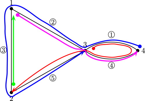
For example, trail ${\mathsf{T}}_3$ from Fig. 3 starts at 3 and ends at 2, as the lemma requires, since the product of the transposition sequence pictured in Fig. 3 is $(4,3,2,1)$.

Fig. 3 Graph from Fig. 1 with its MIGTs.

Definition 5.2

Given a labeled graph $\mathit{G}$, by ${\mathit{G}}^{\prime }$, the Graph Dual, we mean the following labeled graph:

–	The vertices of ${\mathit{G}}^{\prime }$ are the same as those of $\mathit{G}$.
–	The edges of ${\mathit{G}}^{\prime }$ are determined as follows: For any vertices $x$ and $y$, if the edge labeled $k$ in $\mathit{G}$ is used by both trail ${\mathsf{T}}_x$ and trail ${\mathsf{T}}_y$, then make an edge labeled $k$ between $x$ and $y$.

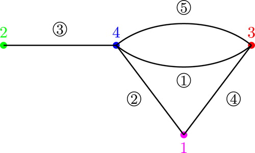
For example, consider the graph of Fig. 3, with its MIGTs displayed. Since ${\mathsf{T}}_1$ and ${\mathsf{T}}_3$ both use edge $4$, the Graph Dual will have an edge with label $4$ between vertices 1 and 3; the full Graph Dual is shown in Fig. 4. Notice that the Algebraic Dual from Example 2.2 viewed as a graph is exactly the graph in Fig. 4. In the next theorem we point out that this is always true.

Fig. 4 Graph Dual of the graph from Fig. 3.

Theorem 5.3

For any transposition sequence, its Algebraic Dual is the same as its Graph Dual.

Proof

Suppose the transposition sequence is $〈{\mathsf{s}}_{\mathsf{1}},\dots ,{\mathsf{s}}_{\mathsf{m}}〉$, with Algebraic Dual $〈{\mathsf{s}}_{\mathsf{1}}^{\prime },\dots ,{\mathsf{s}}_{\mathsf{m}}^{\prime }〉$, and Graph Dual $〈{\mathsf{t}}_{\mathsf{1}},\dots ,{\mathsf{t}}_{\mathsf{m}}〉$. We show that for any $k$, ${\mathsf{t}}_{\mathsf{k}}={\mathsf{s}}_{\mathsf{k}}^{\prime }$. Supposing ${\mathsf{s}}_{\mathsf{k}}=(x,y)$ and $\alpha ={\mathsf{s}}_{\mathsf{1}}\cdots {\mathsf{s}}_{\mathsf{k-1}}$, then by Lemma 2.6 ${\mathsf{s}}_{\mathsf{k}}^{\prime }=(x^{\prime },y^{\prime })$, where $x^{\prime }={\alpha }^{-1}\left(x\right)$ and $y^{\prime }={\alpha }^{-1}\left(y\right)$. Consider the MIGTs of the labeled graph $〈{\mathsf{s}}_{\mathsf{1}},\dots ,{\mathsf{s}}_{\mathsf{k}-\mathsf{1}}〉$; by Lemma 5.1, ${\mathsf{T}}_{x^{\prime }}$ starts at $x^{\prime }$ and ends at $x$, and ${\mathsf{T}}_{y^{\prime }}$ starts at $y^{\prime }$ and ends at $y$. Thus when edge ${\mathsf{s}}_{\mathsf{k}}$ is added to the graph, ${\mathsf{T}}_{x^{\prime }}$ is extended by moving along the edge labeled $k$ to now end at $y$, while ${\mathsf{T}}_{y^{\prime }}$ is extended by moving along the edge labeled $k$ to now end at $x$. So ${\mathsf{t}}_{\mathsf{k}}=(x^{\prime },y^{\prime })={\mathsf{s}}_{\mathsf{k}}^{\prime }$, and we are done.□

Since the Algebraic Dual and the Graph Dual are the same, we may use the term dual to refer to either of the equivalent notions.

6 Goulden-Yong Dual

In [3], they define a dual that applies only to trees, using topological methods. When restricted to trees, we show that their dual is the same as our dual, and thus our bijection is in fact the same as that of [3].

Definition 6.1

[3] Given a labeled tree $\mathit{T}$ on $n$ vertices, its Circle Chord Diagram, is the following structure:

A circle, together with $n$ distinct points on the circle, labeled by the numbers $1,\dots ,n$, in the clockwise direction, drawing a chord between $x$ and $y$ if there is an edge between $x$ and $y$ in $\mathit{T}$.

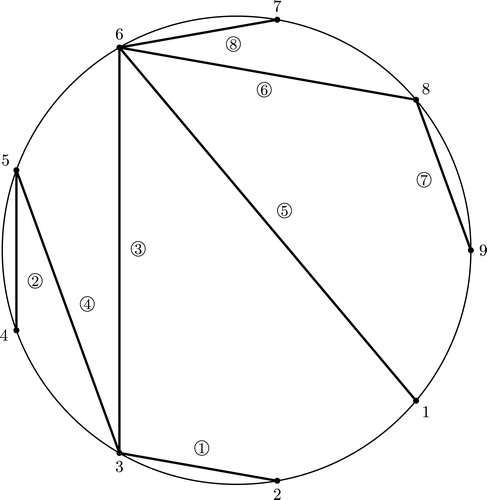
Consider the tree shown in Fig. 5 (it is the same as the example in [3]); its MIGTs are drawn in, but can be ignored for now. The Circle Chord Diagram for the tree of Fig. 5 is shown in Fig. 6. Notice that the chords in Fig. 6 are non-crossing, i.e. any two chords either do not meet, or only meet at a vertex on the circle. For a tree with $n$ vertices and non-crossing chords, its Circle Chord Diagram has the following properties:

Fig. 5 A tree from ${\mathcal{F}}^{(9\dots 1)}$ and its MIGTs.

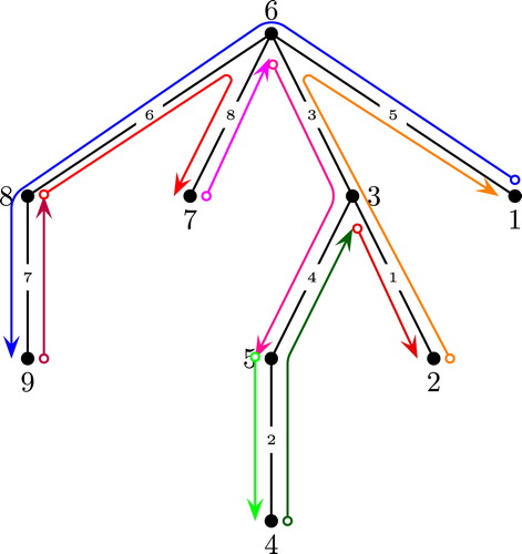
Fig. 6 Circle Chord Diagram of the tree in Fig. 5.

–	The $n$ vertices on the circle, break up the circle into $n$ arcs, i.e. the arc between $1$ and $2$ (we call arc 2), the arc between $2$ and $3$ (we call arc 3), and so on, calling the arc between $n$ and $1$, arc 1.
–	The chords break up the region inside the circle into $n$ regions, each containing one of the $n$ arcs; we refer to the region with arc $k$ as region $k$.

In [3], multiplication in ${\mathbf{S}}_n$ is from right-to-left, however their labeling of the transpositions in a transposition sequence increases from left-to-right. We wanted both the labeling and the multiplication to go in the same order. To make our work fit most smoothly with their work, notice that we have opted to keep their labeling from left-to-right, but have changed multiplication to also go from left-to-right. Thus in [3], when they refer to factorizations of $(1,2,\dots ,n)$ into$n-1$ transpositions, in our terminology, they are referring to exactly the set ${\mathcal{F}}^{(n\dots 1)}$ from Definition 1.2. Recall that from Theorem 4.1 we know that the transpositions sequences in ${\mathcal{F}}^{(n\dots 1)}$ are trees. Thus it makes sense to find the Circle Chord Diagram of a transposition sequence from ${\mathcal{F}}^{(n\dots 1)}$. In [3] (see Theorem 2.2) the following theorem is proved.

Theorem 6.2

[3] For any transposition sequence $\mathbf{s}\in {\mathcal{F}}^{(n\dots 1)}$ its Circle Chord Diagram has the following properties:

1.	The chords are non-crossing.
2.	At each of the $n$ vertices on the circle, the labels of the incident chords decrease as we turn clockwise.

The properties of the theorem can all be verified of the example in Fig. 6; for example, at vertex 3, turning clockwise, we encounter decreasing labels: 4, then 3, then 1. We now give a definition that basically comes from [3], calling it the Goulden–Yong Dual; the coherence of the definition depends on Theorem 6.2.

Definition 6.3

[3] Given a tree from ${\mathcal{F}}^{(n\dots 1)}$, its Goulden–Yong Dual is determined as follows:

–	Draw its Circle Chord Diagram, which divides the disk into $n$ regions.
–	Place a new vertex in each region, labeling the vertex $k$ if it is in the region that contains arc $k$.
–	Create an edge between two new vertices if their regions have a chord in common, labeling the edge by the label on the chord.

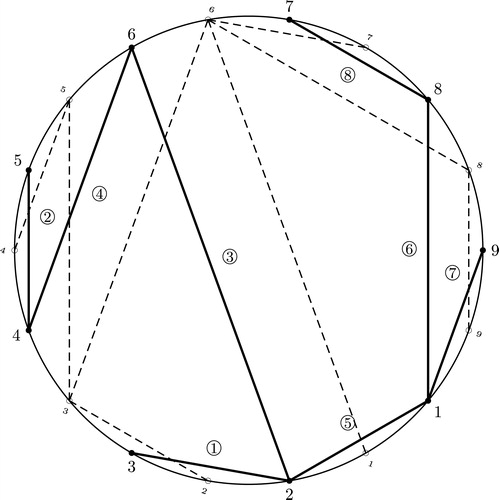
For example, the Goulden–Yong Dual of the tree in Fig. 5 is pictured in Fig. 7: The dashed edges and smaller vertices depict the original tree from the Circle Chord Diagram of Fig. 6, and the solid lines with larger vertices depict its Goulden–Yong Dual. Note that the Graph Dual of the tree in Fig. 5 is exactly the Goulden–Yong Dual pictured in Fig. 7; we will see that this is generally true in Theorem 6.5. As an example of the next lemma, note that the chords of region $2$ of Fig. 6 are the ones labeled $1$, $3$, and $5$, exactly the same as the edges traversed by trail ${\mathsf{T}}_2$.

Fig. 7 Goulden–Yong Dual (Solid Lines) of the tree in Figs. 5 and 6 (Dashed Lines).

Lemma 6.4

Suppose $\mathit{T}\in {\mathcal{F}}^{(n\dots 1)}$ and$C$ is its Circle Chord Diagram. Suppose $x\in \left[n\right]$. Then the edges in ${\mathsf{T}}_x$ are exactly the edges on the boundary in region $x$ of $C$.

Proof

Suppose the vertices of trail ${\mathsf{T}}_x$, in order, are $x,x_1,\dots ,x_k$. Let $e$ be the most clockwise edge at $x$ (for example, in Fig. 6, edge $3$ is the most clockwise edge at vertex $6$). By property 2. of Theorem 6.2, ${\mathsf{T}}_x$ moves along edge $e$ from $x$ to $x_1$. Then, again by property 2., the trail goes from $x_1$ to $x_2$, along the edge that is one chord counter-clockwise from $e$, when turning at $x_1$ (for example, in Fig. 6, at vertex $3$, the chord labeled by $4$ is one chord counter-clockwise from the chord labeled $3$). As we continue we see that ${\mathsf{T}}_x$ traverses one of the $n$ regions of $C$, moving along its boundary in a clockwise fashion, starting at $x$ on the circle and ending at $x-1$ (understanding vertex $0$ to be the same as vertex $n$). That is, ${\mathsf{T}}_x$ consists of exactly the edges of region $x$.□

Theorem 6.5

For any tree from ${\mathcal{F}}^{(n\dots 1)}$, its Goulden–Yong Dual is the same as its dual.

Proof

Consider some tree $\mathit{T}\in {\mathcal{F}}^{(n\dots 1)}$, and let $C$ be its Circle Chord Diagram. Let ${\mathit{T}}^{\prime }$ be its Graph Dual and ${\mathit{T}}^{\ast }$ its Goulden–Yong Dual. Both ${\mathit{T}}^{\prime }$ and ${\mathit{T}}^{\ast }$ are labeled graphs with vertex set $\left[n\right]$, so it suffices to observe that for any distinct $u,v\in \left[n\right]$, we have the following equivalences (where the second one follows by Lemma 6.4).

$\text{In}{\mathit{T}}^{\prime }\text{there is an edge labeled}k\text{between}u\text{and}v$. $$\iff {\mathsf{T}}_u\text{and}{\mathsf{T}}_v\text{both use edge}k$$ $$\iff \text{Chord}k\text{is on the boundary of region}u\text{and region}v.$$ $$\iff \text{In}{\mathit{T}}^{\ast }\text{there is an edge labeled}k\text{between}u\text{and}v.\square$$

7 Realizability

One of the central ideas of this paper is to create a labeled graph from a transposition sequence, and then consider the relevant trails, namely the MIGTs. Thus a natural question in this context is to consider systems of trails on unlabeled graphs (formalized in Definition 7.1), and ask which ones arise as MIGTs. The main result of this section is Theorem 7.6, which exactly characterizes the systems of trails that arise as MIGTs. This section is not necessary for the alternate proof of the Goulden–Yong result; instead, it provides a further investigation of the tools used in this paper.

Definition 7.1

A Trail Double Cover of a graph is a set of trails such that:

–	A unique trail begins at each vertex, and
–	Every edge of the graph is used by exactly two trails.

An example of a Trail Double Cover can be seen in Fig. 3. The next lemma shows that Definition 7.1 is interesting: it is a natural definition, which includes systems of trails that arise from MIGTs.

Lemma 7.2

The set of MIGTs of a labeled graph is a Trail Double Cover.

Proof

For the first requirement on being a Trail Double Cover, we note that there is only one MIGT trail that starts at a vertex, since there is at most one smallest edge at a vertex.

We proceed by induction on the number of edges to prove the second requirement: that each edge is used by exactly two trails. Let our graph be $\mathit{G}$. For the inductive step, remove the edge $\overline{1}$, i.e. the edge labeled by 1; call the resulting graph ${\mathit{G}}^{-}$. Suppose edge $\overline{1}$ in graph $\mathit{G}$ consists of vertices $x$ and $y$. By inductive hypothesis, in ${\mathit{G}}^{-}$, every edge is used by exactly two trails; the fact that the edge labels of ${\mathit{G}}^{-}$ start at $2$ instead of $1$, has no effect on the argument. Define ${\mathsf{T}}_x^{-}$ to be the trail ${\mathsf{T}}_x$ in ${\mathit{G}}^{-}$, and ${\mathsf{T}}_y^{-}$ to be ${\mathsf{T}}_y$ in ${\mathit{G}}^{-}$. Thus in $\mathit{G}$, ${\mathsf{T}}_x$ starts at $x$, follows edge $\overline{1}$ to $y$ and then does exactly what ${\mathsf{T}}_y^{-}$ does in ${\mathit{G}}^{-}$. Likewise, in $\mathit{G}$, ${\mathsf{T}}_y$ goes from $y$ to $x$ and then follows ${\mathsf{T}}_x^{-}$. The rest of the trails of $\mathit{G}$ are the same as those of ${\mathit{G}}^{-}$. Thus $\overline{1}$ is used exactly twice, as are the rest of the edges.□

Definition 7.3

A Trail Double Cover $\mathcal{T}$ is realizable if there is an edge labeling of the graph such that the resulting set of MIGT trails is $\mathcal{T}$.

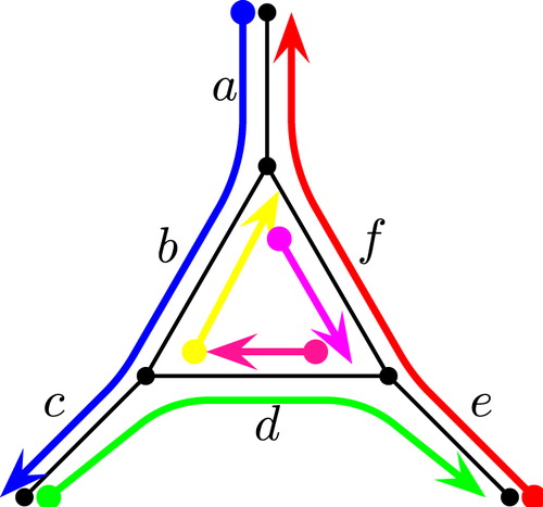
By definition, the Trail Double Cover pictured in Fig. 3 is realizable. However the Trail Double Cover pictured in Fig. 8 is not realizable; this point can be checked directly, however, we will see that this follows from Theorem 7.6. Though the Trail Double Cover of Fig. 8 is not realizable, we can still see any Trail Double Cover as representing a permutation of its vertices: each trail maps its start vertex to its end vertex. We can view a Trail Double Cover in this way because a unique trail begins at each vertex, and as the next lemma shows, a unique trails ends at each vertex.

Fig. 8 A Trail Double Cover that is not realizable.

Lemma 7.4

In any Trail Double Cover, each vertex of the graph is the final vertex of a unique trail.

Proof

If the graph has $n$ vertices, then the Trail Double Cover has $n$ trails that start at those $n$ vertices. So it suffices to show that each vertex is the final vertex of some trail. Suppose, for contradiction, that there were a vertex $v$ which was not the final vertex of any trail. Then the trail that starts at $v$ contains an odd number of edges incident to $v$, and any other trail contains an even number of edges incident to $v$. This implies that in total, an odd number of edges incident to $v$ are in use by some trail, however, this contradicts the property that in a Trail Double Cover, each edge incident to $v$ is in use by exactly two trails.□

We give a characterization of realizability using an auxiliary digraph (i.e. directed graph). Edges in a digraph are called arcs; we will refer to the arc that starts at vertex $x$ and goes to vertex $y$ by $\overrightarrow{(x,y)}$. In a digraph, we refer to a directed trail as a trail that always moves in the direction of the arcs. From a Trail Double Cover we will create an auxiliary digraph by converting each one of the trails in the Trail Double Cover into a directed trail in a new digraph.

Definition 7.5

Given any Trail Double Cover $\mathcal{T}$ on $\mathit{G}$, we define its Edge Digraph to be the following digraph:

–	Its vertices are the edges of $\mathit{G}$.
–	For each trail $〈v_1,e_1,v_2,e_2,\dots ,v_k,e_k,v_{k+1}〉$ in $\mathcal{T}$, we have the following arcs: $$\overrightarrow{(e_1,e_2)},\overrightarrow{(e_2,e_3)},\dots ,\overrightarrow{(e_{k-1},e_k)}.$$

For example, Fig. 9 is the Edge Digraph of the Trail Double Cover in Figs. 3, and 10 is the Edge Digraph of Fig. 8. The next theorem gives us a criterion for determining whether or not a Trail Double Cover is realizable. Applying the theorem to the Trail Double Cover of Fig. 8, we see that it is not realizable, since its Edge Digraph, drawn in Fig. 10, does have a directed cycle.

Fig. 9 The Edge Digraph of the Trail Double Cover in Fig. 3.

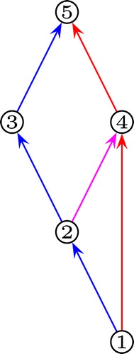
Fig. 10 The Edge Digraph of the Trail Double Cover in Fig. 8.

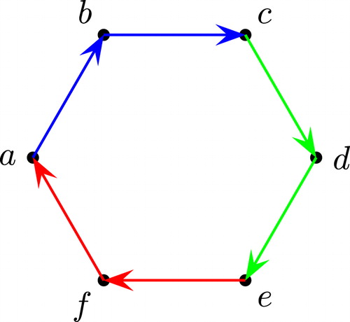
Fig. 11 The configuration of trails in the neighborhood of a vertex.

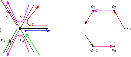
Theorem 7.6

A Trail Double Cover is realizable if and only if its Edge Digraph has no directed cycle.

Proof

Suppose $\mathit{G}$ is the graph and $\mathcal{T}$ is a Trail Double Cover on it. Let $\mathit{D}$ be the Edge Digraph of $\mathcal{T}$.

Forward Direction: Consider an edge labeling that yields $\mathcal{T}$. Any arc of $\mathit{D}$ goes from $e_1$ to $e_2$, where $e_1$ and $e_2$ are edges of $\mathit{G}$ such that the label of $e_1$ is less than the label of $e_2$. So $\mathit{D}$ cannot have a directed cycle.

Backwards Direction: Supposing $\mathit{D}$ has no directed cycle, take any topological sort of $\mathit{D}$ to arrive at an edge labeling of $\mathit{G}$. For example, the graph of Fig. 3 has the edge digraph in Fig. 9, so one topological sort is 1, 2, 3, 4, 5, which corresponds to the original edge labeling of the graph in Fig. 3, while the other topological sort is 1, 2, 4, 3, 5, giving a different edge labeling of the graph in Fig. 3. Let ${\mathit{G}}^{\ast }$ be $\mathit{G}$ with its edges labeled according to the topological sort. We show that the set of MIGTs of ${\mathit{G}}^{\ast }$ is exactly $\mathcal{T}$. For any Trail Double Cover, at each vertex $x$ we get the situation shown in Fig. 11 (left side): One trail, say ${\mathsf{T}}_1$, starts at $x$ by using edge $e_1$, one trail, say ${\mathsf{T}}_d$, ends at $x$ by using edge $e_d$, and the rest of the trails enter $x$ by using one edge and leave by another. We let ${\mathsf{T}}_{(i,i+1)}$ refer to the trail that enters along $e_i$ and leaves along $e_{i+1}$, for $i=1,2,\dots ,d-1$. It is possible that some of the $d+1$ trails ${\mathsf{T}}_1,{\mathsf{T}}_d,{\mathsf{T}}_{(1,2)},{\mathsf{T}}_{(2,3)},\dots ,{\mathsf{T}}_{(d-1,d)}$ are not distinct, and any $e_i$ and $e_j$ might be multi-edges attaching the same two vertices. The related part of $\mathit{D}$ is pictured in Fig. 11 (right side). In our topological sort we must have $e_1<e_2<\cdots <e_d$. Now, consider any trail $\mathsf{T}=〈v_1,w_1,v_2,\dots ,v_{k-1},w_{k-1},v_k〉$ in $\mathcal{T}$; we show that in the topological ordering of the edges, $\mathsf{T}$ is an MIGT in ${\mathit{G}}^{\ast }$. Referring to Fig. 11 (left side), we can see that edge $w_1$ of $\mathsf{T}$, being its first edge corresponds to an edge like $e_1$ of Fig. 11 (right side) and so it is the smallest edge incident to $v_1$, as required. Similarly, edge $w_{k-1}$ of $\mathsf{T}$ corresponds to edge like $e_d$, and so it is the largest labeled edge at $v_k$, as required. Consider any intermediate edges $w_i$ and $w_{i+1}$ of $\mathsf{T}$, both incident to vertex $v_{i+1}$; these edges correspond to some $e_j$ and $e_{j+1}$ in Fig. 11. We suppose the trail has been MIGT up to and including $w_i$, and show that it still is for $w_{i+1}$. The topological ordering of the edges pictured in Fig. 11 (right side) indicates that $w_{i+1}$ is the next largest labeled edge, so this matches the MIGT. Thus we have shown that every trail of $\mathcal{T}$ is an MIGT in ${\mathit{G}}^{\ast }$. Also note that every MIGT of ${\mathit{G}}^{\ast }$ is in $\mathcal{T}$ since being a Trail Double Cover, $\mathcal{T}$ used every edge twice, so there can be no more MIGTs. Thus $\mathcal{T}$ is exactly the set of MIGTs on ${\mathit{G}}^{\ast }$, so we have realized $\mathcal{T}$.□

8 Conclusion and future work

In this paper we focused on minimal transitive factorizations of the permutation $(n,\dots ,2,1)$, investigating an interesting bijection. In [2] a general formula is found for the number of minimal transitive factorizations of any permutation. Based on this result, they motivate the search for interesting bijections between such sets of factorizations and other sets of combinatorial interest. Making progress on this program, [10] found a bijection for the minimal transitive factorizations of $\left(1\right)(2,\dots ,n)$, and [11] found bijections for $(1,2)(3,\dots ,n)$ and $(1,2,3)(4,\dots ,n)$; both papers used parking functions. Our hope is that our alternative definitions of the dual, which apply to any graph (not just trees), could be a useful tool for such research.

Acknowledgments

I acknowledge and thank Nikos Apostolakis for his role in this paper. We began working on this project together, but decided to publish our results separately, with different emphases. Thus, all of the results in this paper come out of discussion and work with Nikos Apostolakis. Furthermore, I thank him for having made all the figures that appear in this paper. His paper that came out of our joint work is submitted and under review, and can be found at the arXiv [12]. His paper includes his interpretation and exposition of our joint work, as well as his individual contributions beyond that.

My work was supported by a PSC-CUNY Research Award (Traditional A).

References

- DénesJ., The representation of a permutation as the product of a minimal number of transpositions, and its connection with the theory of graphs Magyar Tud. Akad. Mat. Kutató Int. Közl. 41959 63–71
- GouldenI.P.JacksonD.M., Transitive factorisations into transpositions and holomorphic mappings on the sphere Proc. Amer. Math. Soc. 125 1 1997 51–60
- GouldenI.YongA., Tree-like properties of cycle factorizations J. Combin. Theory Ser. A 98 1 2002 106–117
- ArnoldV., Topological classification of trigonometric polynomials and combinatorics of graphs with an equal number of vertices and edges Funct. Anal. Appl. 30 1 1996 1–14
- GouldenI.P.JacksonD.M.VakilR., The Gromov-Witten potential of a point, Hurwitz numbers, and Hodge integrals Proc. Lond. Math. Soc. (3) 83 3 2001 563–581
- E. Duchi, D. Poulalhon, G. Schaeffer, Bijections for simple and double Hurwitz numbers,arXiv:1410.6521v1.
- MoszkowskiP., A solution to a problem of Dénes: a bijection between trees and factorizations of cyclic permutations European J. Combin. 10 1 1989 13–16
- GouldenI.P.PepperS., Labelled trees and factorizations of a cycle into transpositions Discrete Math. 113 1–3 1993 263–268
- MartínM.C.H., Complejidad de Estructuras Geométricas y Combinatorias(Ph.D. thesis)1999Universitat Politècnica de Catalunya
- KimD.SeoS., Transitive cycle factorizations and prime parking functions J. Combin. Theory Ser. A 104 1 2003 125–135
- RattanA., Permutation factorizations and prime parking functions Ann. Comb. 10 2 2006 237–254
- N. Apostolakis, A duality for labeled graphs and factorizations with applications to graph embeddings and Hurwitz enumeration, arXiv eprints:1804.01214v4 (April 2018).