On the radio number for corona of paths and cycles

Abstract

Radio $k$-coloring of graphs is one of the variations of frequency assignment problem. For a simple connected graph $G$ and a positive integer $k⩽diam\left(G\right)$, a radio $k$-coloring is an assignment $f$ of positive integers (colors) to the vertices of $G$ such that for every pair of distinct vertices $u$ and $v$ of $G$, the difference between their colors is at least $1+k-d(u,v)$. The maximum color assigned by $f$ is called its span, denoted by $r{c}_k\left(f\right)$. The radio $k$-chromatic number $r{c}_k\left(G\right)$ of $G$ is $min\{r{c}_k\left(f\right):f\text{is a radio}k\text{-coloring of}G\}$. If $d$ is the diameter of $G$, then a radio $d$-coloring is referred as a radio coloring and the radio $d$-chromatic number as the radio number, denoted by $rn\left(G\right)$, of $G$. The corona $G\odot H$ of two graphs $G$ and $H$ is the graph obtained by taking one copy of $G$ and $\left|V\left(G\right)\right|$ copies of $H$, and joining each and every vertex of the $i^{\text{th}}$ copy of $H$ with the $i^{\text{th}}$ vertex of $G$ by an edge. In this paper, for path $P_n$ and cycle $C_m$, $m\ge 5$, we determine $rn(P_n\odot C_m)$ when $n$ is even, and give an upper bound for the same when $n$ is odd. Also, for $m\ge 4$, we determine the radio number of $P_n\odot P_m$ when $n$ is even, and give both upper and lower bounds for $rn(P_n\odot P_m)$ when $n$ is odd.

Keywords:

• Radio $k$-coloring
• Radio $k$-chromatic number
• Radio coloring
• Radio number

1 Introduction

The problem of obtaining an assignment of frequencies to transmitters in some optimal manner is said to be Frequency Assignment Problem (FAP). Due to rapid growth of wireless networks and to the relatively scarce radio spectrum, the importance of FAP is growing significantly. One of the FAPs is the problem of assigning radio frequencies to transmitters at different locations without causing interference and reducing maximum frequency used. Hale [1] has modeled FAP as graph labeling problem as follows. Transmitters are represented by vertices of a graph and those vertices corresponding to very close transmitters are joined by edges. Maximum interference occurs among transmitters corresponding to adjacent vertices. Now, assigning frequencies to transmitters is same as assigning positive integers (colors) to vertices.

Motivated by channel assignment to radio stations, Chartrand et al. [2] have introduced radio $k$-coloring of graphs. For a simple connected graph $G$ and an integer $k$, $1⩽k⩽diam\left(G\right)$, a radio $k$-coloring of $G$ is an assignment $f$ of positive integers to the vertices of $G$ such that $|f\left(u\right)-f\left(v\right)|⩾1+k-d(u,v)$ for all distinct vertices $u$ and $v$ of G. The maximum color assigned by $f$ is called the span of $f$, denoted by $r{c}_k\left(f\right)$. The radio $k$-chromatic number $r{c}_k\left(G\right)$ of $G$ is the minimum of spans over all radio $k$-colorings of $G$. A radio $k$-coloring $f$ of $G$ with span $r{c}_k\left(G\right)$ is referred as a minimal radio $k$-coloring of $G$. For some special values of $k$, there are some special names of radio $k$-colorings and as well as radio $k$-chromatic numbers in the literature. A radio $1$-coloring is a proper coloring of $G$ and $r{c}_1\left(G\right)=\chi \left(G\right)$. If $k=d$, the diameter of $G$, then a radio $d$-coloring is called a radio coloring and the radio $d$-chromatic number is said to be the radio number. Radio $(d-1)$-coloring and radio $(d-2)$-coloring are called antipodal coloring and nearly antipodal coloring respectively. The radio $(d-1)$-chromatic number and the radio $(d-2)$-chromatic number are called the antipodal number and the nearly antipodal number respectively.

If we see the literature of radio $k$-coloring for operation between graphs, it is studied only for Cartesian product of graphs. Even though, radio $k$-coloring is defined for $k⩽diam\left(G\right)$, some authors have studied it for $k⩾diam\left(G\right)$ as it is useful in finding radio $k$-chromatic number of larger graphs. Kchikech et al. [3] have given lower and upper bounds for $r{c}_k(P_n\square P_n)$ when $k⩾2n-3$. Also, they have given an upper bound for radio $k$-chromatic number of Cartesian product of two arbitrary graphs. Kim et al. [4] have determined the radio number of Cartesian product of path $P_n$ and complete graph $K_m$ as $\frac{m{n}^2-2n+4}{2}$ if $n$ is even and $\frac{m{n}^2-2n+m+4}{2}$ if $n$ is odd. Ajayi and Adefokun [5] have given bounds for the radio number for Cartesian product of path and star. Morris-Rivera [6] has determined that $rn(C_n\square C_n)$ is $2p^3+4p^2-p$ if $n=2p$ and is $2p^3+4p^2+2p+1$ if $n=2p+1$. Saha and Panigrahi [7] found the exact value of radio number of $C_m\square C_n$, toroidal grid, when at least one of $m$ and $n$ is even. Kola and Panigrahi [8] have given a lower bound for $r{c}_k\left(G\right)$ for an arbitrary graph $G$ and using this lower bound, they have given a lower bound for radio $k$-chromatic number of prism graph $C_n\square P_m$. Further, they proved this lower bound is exact for the radio number of $C_n\square P_2$, when $n\equiv 1mod4$ and $n\equiv 2mod8$. The corona $G\odot H$ of two graphs $G$ and $H$ is the graph obtained by taking one copy of $G$ and $\left|V\left(G\right)\right|$ copies of $H$, and joining each and every vertex of the $i\text{th}$ copy of $H$ with the $i\text{th}$ vertex of $G$ by an edge. It is easy to see that $G\odot H\ncong H\odot G$ if $G\ncong H$. Also, $diam(G\odot H)=diam\left(G\right)+2$.

In this article, for $m\ge 5$, we determine the radio number for $P_n\odot C_m$ when $n$ is even and we give lower and upper bounds for $rn(P_n\odot C_m)$ when $n$ is odd. Also, for $m\ge 4$, we determine $rn(P_n\odot P_m)$ when $n$ is even and give lower and upper bounds for the same when $n$ is odd.

2 Results

We use the following definition and lemma to get the span of a radio coloring.

Definition 2.1

For a graph $G$ of order $n$ and a radio $k$-coloring $f$ of $G$, let $x_1,x_2,x_3,\dots ,x_n$ be an ordering of vertices of $G$ such that $f\left(x_i\right)\le f\left(x_{i+1}\right)$, $1\le i\le n-1$. We define ${ϵ}_i=f\left(x_i\right)-f\left(x_{i-1}\right)-(1+k-d(x_i,x_{i-1}))$, $2\le i\le n$.

Lemma 2.2

For any radio $k$ -coloring $f$ of a graph $G$ of order $n$ , $$r{c}_k\left(f\right)=(n-1)(1+k)-\sum _{i=2}^{n}d(x_i,x_{i-1})+\sum _{i=2}^n{ϵ}_i+1$$ where $x_i$ s are as given in Definition 2.1 .

Proof

$$f\left(x_n\right)-f\left(x_1\right)=\sum _{i=2}^n[f\left(x_i\right)-f\left(x_{i-1}\right)]=\sum _{i=2}^n[1+k-d(x_i,x_{i-1})+{ϵ}_i]=(n-1)(1+k)-\sum _{i=2}^{n}d(x_i,x_{i-1})+\sum _{i=2}^n{ϵ}_i.$$ Since $f\left(x_1\right)=1$, $r{c}_k\left(f\right)=f\left(x_n\right)=(n-1)(1+k)-{\sum }_{i=2}^{n}d(x_i,x_{i-1})+{\sum }_{i=2}^n{ϵ}_i+1$. ■

To get a lower bound for the radio number of the graph under discourse, we use the lower bound technique for radio $k$-coloring given by Das et al. [9]. For a subset $S$ of the vertex set of a graph $G$, let $N\left(S\right)$ be the set of all vertices of $G$ adjacent to at least one vertex of $S$.

Theorem 2.3

[9] If $f$ is a radio $k$ -coloring of a graph $G$ , then $$r{c}_k\left(f\right)\ge \left|D_k\right|-2p+2\sum _{i=0}^p\left|L_i\right|(p-i)+\alpha +\beta ,$$ where $D_k$ and $L_i$ ’s are defined as follows. If $k=2p+1$ , then $L_0=V\left(C\right)$ , where $C$ is a maximal clique in $G$ . If $k=2p$ , then $L_0=\left\{v\right\}$ , where $v$ is a vertex of $G$ . Recursively define $L_{i+1}=N\left(L_i\right)\setminus (L_0\cup L_1\cup \cdots \cup L_i)$ for $i=0,1,2,\dots ,p-1$ . Let $D_k=L_0\cup L_1\cup \cdots \cup L_p$ . The minimum and the maximum colored vertices among the vertices of $D_k$ are in $L_{\alpha }$ and $L_{\beta }$ respectively.

As a direct consequence of Theorem 2.3, we have the theorem below.

Theorem 2.4

For any graph $G$ and $1\le k\le diam\left(G\right)$ , we have $$r{c}_k\left(G\right)\ge \left\{\begin{array}{cc}\left|D_k\right|-2p+2\sum _{i=0}^p\left|L_i\right|(p-i)\hfill & ifk=2p+1,\hfill \\ \left|D_k\right|-2p+2\sum _{i=0}^p\left|L_i\right|(p-i)+1\hfill & ifk=2p.\hfill \end{array}\right.$$

Following theorem gives an upper bound for the radio number of corona of path and cycle $P_n\odot C_m$. We refer the condition in the definition of radio $k$-coloring as radio $k$-coloring condition.

Theorem 2.5

For $m\ge 5$ , $$rn(P_n\odot C_m)\le \left\{\begin{array}{cc}(2m+2)p^2+2p\hfill & ifn=2p,\hfill \\ (2m+2)p^2+(2m+4)p+m+2+(\frac{m}{2}-1)p,\hfill & ifn=2p+1andmiseven,\hfill \\ (2m+2)p^2+(2m+4)p+m+2+\left(\frac{m-1}{2}\right)p,\hfill & ifn=2p+1andmisodd.\hfill \end{array}\right.$$

Proof

To give an upper bound for the radio number, we define a radio coloring of $P_n\odot C_m$. Let $v_1{v}_2{v}_3\dots v_n$ be the path $P_n$ and for $i=1,2,3,\dots ,n$, let $C_m^i$ be the copy of $C_m$ in $P_n\odot C_m$ corresponding to the vertex $v_i$ of $P_n$.

Case 1: Let $n=2p$. To give a radio coloring, we first order the vertices of $P_n\odot C_m$ as follows. Let $x_1=v_p$. We label the vertices of $C_m^{n+1-i}$, $i=1,2,3,\dots ,p$, as $x_2,x_4,x_6,\dots ,x_{mn}$ starting from the vertices of $C_m^n$ and once all vertices of $C_m^n$ are labeled, we label the vertices of $C_m^{n-1}$ and so on, in such a way that $d(x_i,x_{i+2})>1$ for $i=2,4,6,\dots ,mn-2$. We label the vertices $v_n,v_{n-1},v_{n-2},\dots ,v_{p+1}$ as $x_{mn+2},x_{mn+4},x_{mn+6},\dots ,x_{mn+n}$ respectively. Now, we label the vertices of $C_m^{p+1-i}$, $i=1,2,3,\dots ,p$, as $x_3,x_5,x_7,\dots ,x_{mn+1}$ starting from the vertices of $C_m^p$ and once all vertices of $C_m^p$ are labeled, we label the vertices of $C_m^{p-1}$ and so on, in such a way that $d(x_i,x_{i+2})>1$ for $i=3,5,7,\dots ,mn-1$. Finally, we label the vertices $v_{p-1},v_{p-2},v_{p-3},\dots ,v_1$ as $x_{mn+3},x_{mn+5},x_{mn+7},\dots ,x_{mn+n-1}$ respectively.

Now, we define a coloring $f$ by $f\left(x_1\right)=1$ and for $i=2,3,4,\dots ,mn+n$, $f\left(x_i\right)=f\left(x_{i-1}\right)+1+(2p+1)-d(x_i,x_{i-1})$. Next, we show that $f$ is a radio coloring of $P_n\odot C_m$ with span $(2m+2)p^2+2p$. By definition of $f$, $x_i$ satisfies radio coloring condition with $x_{i+1}$. Also it is easy to see that $f\left(x_i\right)-f\left(x_{i+3}\right)\ge 2p+1=1+(2p+1)-1\ge 1+(2p+1)-d(x_i,x_{i+3})$. So, it remains to check the radio coloring condition for $x_i$ and $x_{i+2}$. Suppose that $x_i$ and $x_{i+2}$ are on the same copy of $C_m$. Then by the ordering, $d(x_i,x_{i+2})=2$ and $d(x_i,x_{i+1})=d(x_{i+1},x_{i+2})=p+2$. Therefore, $$f\left(x_{i+2}\right)-f\left(x_i\right)=f\left(x_{i+2}\right)-f\left(x_{i+1}\right)+f\left(x_{i+1}\right)-f\left(x_i\right)=p+p=1+(2p+1)-d(x_i,x_{i+2}).$$ Suppose that $x_i$ and $x_{i+2}$ are on different copies of $C_m$. Then $d(x_i,x_{i+2})=3$ and one of $d(x_i,x_{i+1})$ and $d(x_{i+1},x_{i+2})$ is $p+2$ and the other is $p+1$. Therefore, $$f\left(x_{i+2}\right)-f\left(x_i\right)=f\left(x_{i+2}\right)-f\left(x_{i+1}\right)+f\left(x_{i+1}\right)-f\left(x_i\right)=2(1+(2p+1))-d(x_i,x_{i+1})-d(x_{i+1},x_{i+2})=2p+1>1+(2p+1)-d(x_i,x_{i+2}).$$ Suppose that $x_i$ is on a copy of $C_m$ and $x_{i+2}$ is on $P_n$. Then $i=mn$ or $i=mn+1$. If $i=mn$, then $d(x_{mn},x_{mn+2})=p$, $d(x_{mn},x_{mn+1})=p+2$ and $d(x_{mn+1},x_{mn+2})=2p$. Therefore, $$f\left(x_{mn+2}\right)-f\left(x_{mn}\right)=f\left(x_{mn+2}\right)-f\left(x_{mn+1}\right)+f\left(x_{mn+1}\right)-f\left(x_{mn}\right)=p+2=1+(2p+1)-d(x_{mn},x_{mn+2}).$$ If $i=mn+1$, then $d(x_{mn+1},x_{mn+3})=p-1$, $d(x_{mn+1},x_{mn+2})=2p$ and $d(x_{mn+2},x_{mn+3})=p+1$. Therefore, $$f\left(x_{mn+3}\right)-f\left(x_{mn+1}\right)=f\left(x_{mn+3}\right)-f\left(x_{mn+2}\right)+f\left(x_{mn+2}\right)-f\left(x_{mn+1}\right)=p+3=1+(2p+1)-d(x_{mn+1},x_{mn+3}).$$ Suppose that $x_i$ is on path $P_n$ and $x_{i+2}$ is on a copy of $C_m$. Then $i=1$, $d(x_1,x_3)=1$, $d(x_1,x_2)=p+1$ and $d(x_2,x_3)=p+2$. Therefore, $$f\left(x_3\right)-f\left(x_1\right)=f\left(x_3\right)-f\left(x_2\right)+f\left(x_2\right)-f\left(x_1\right)=p+1+p=1+(2p+1)-d(x_1,x_3).$$ Suppose both $x_i$ and $x_{i+2}$ are on $P_n$. Then $d(x_i,x_{i+2})=1$ and one of $d(x_i,x_{i+1})$ and $d(x_{i+1},x_{i+2})$ is $p+1$ and the other is $p$. Therefore, $$f\left(x_{i+2}\right)-f\left(x_i\right)=f\left(x_{i+2}\right)-f\left(x_{i+1}\right)+f\left(x_{i+1}\right)-f\left(x_i\right)=2(1+(2p+1))-d(x_i,x_{i+1})-d(x_{i+1},x_{i+2})=2p+3>1+(2p+1)-d(x_i,x_{i+2}).$$

Therefore $f$ is a radio coloring of $P_n\odot C_m$. From the definition of $f$, we have ${\sum }_{i=2}^{mn+n}{ϵ}_i=0$. Since the sequence of distances ${\left\{d(x_i,x_{i-1})\right\}}_{i=2}^{mn+n}$ is such that the $2m$ terms $p+1,p+2,p+2,\dots ,p+2$ repeated $p$ times, that is, up to $d(x_{mn+1},x_{mn})$, $d(x_{mn+2},x_{mn+1})=2p$ and an alternating sequence of $p+1$ and $p$ from $d(x_{mn+3},x_{mn+2})$ to $d(x_{mn+n},x_{mn+n-1})$, we have $$\sum _{i=2}^{mn+n}d(x_i,x_{i-1})=\sum _{i=2}^{mn+1}d(x_i,x_{i-1})+d(x_{mn+2},x_{mn+1})+\sum _{i=mn+3}^{mn+n}d(x_i,x_{i-1})=((p+2)(2m-1)p+(p+1)p)+2p+((p+1)(p-1)+p(p-1))=(2m+2)p^2+4pm-1.$$ Now, by Lemma 2.2, $rn\left(f\right)=(mn+n-1)(2p+1+1)-((2m+2)p^2+4pm-1)+1=(2m+2)p^2+2p$.

Case 2: Let $n=2p+1$ and $m$ be even. As in Case 1, here also first we order the vertices of $P_n\odot C_m$. Let $x_1=v_{p+1}$. We label $x_2,x_4,x_6,\dots ,x_{mn}$ as in Case 1 starting from the vertices of $C_m^n$ ending after labeling $\frac{m}{2}$ vertices of $C_m^{p+1}$. We label the vertices $v_{p+1},v_{p+2},v_{p+3},\dots ,v_n$ as $x_{mn+2},x_{mn+4},x_{mn+6},\dots ,x_{mn+n-1}$ respectively. Now, we label $x_3,x_5,x_7,\dots ,x_{mn+1}$ as in Case $1$ starting from the vertices of $C_m^{p+1}$ ending after labeling all the vertices of $C_m^1$. Finally, we label the vertices $v_1,v_2,v_3,\dots ,v_p$ as $x_{mn+3},x_{mn+5},x_{mn+7},\dots ,x_{mn+n}$ respectively.

Now, we define a coloring $f$ by $f\left(x_1\right)=1$ and for $i=2,3,4,\dots ,mn+n$, $$f\left(x_i\right)=\left\{\begin{array}{cc}f\left(x_{i-1}\right)+1+(2p+2)-d(x_i,x_{i-1})+1,\hfill & \text{if}i\text{is even and}d(x_i,x_{i-1})=p+3,\hfill \\ f\left(x_{i-1}\right)+1+(2p+2)-d(x_i,x_{i-1}),\hfill & \text{otherwise}.\hfill \end{array}\right.$$

Checking the radio coloring condition for $x_i$ and $x_{i+2}$ is similar to the previous case except for the case that both $x_i$ and $x_{i+2}$ are on same copy of $C_m$. Then we have either $d(x_{i+1},x_i)=d(x_{i+1},x_{i+2})=p+2$ or $d(x_{i+1},x_i)=d(x_{i+1},x_{i+2})=p+3$. As in the previous case, we can check the condition if $d(x_{i+1},x_i)=d(x_{i+1},x_{i+2})=p+2$. Suppose that $d(x_{i+1},x_i)=d(x_{i+1},x_{i+2})=p+3$. Since only one of $i+1$ and $i+2$ is even, by the definition of $f$, we have either $f\left(x_{i+1}\right)=f\left(x_i\right)+1+(2p+2)-d(x_{i+1},x_i)+1$ or $f\left(x_{i+2}\right)=f\left(x_{i+1}\right)+1+(2p+2)-d(x_{i+2},x_{i+1})+1$. Therefore, $$f\left(x_{i+2}\right)-f\left(x_i\right)=f\left(x_{i+2}\right)-f\left(x_{i+1}\right)+f\left(x_{i+1}\right)-f\left(x_i\right)=2(1+(2p+2))-d(x_i,x_{i+1})-d(x_{i+1},x_{i+2})+1=2p+1=1+(2p+2)-d(x_i,x_{i+2}).$$ Hence $f$ is a radio coloring. By the definition of $f$, we get ${\sum }_{i=2}^{mn+n}{ϵ}_i=(\frac{m}{2}-1)p$ and by the ordering of vertices, we have ${\sum }_{i=2}^{mn+n}d(x_i,x_{i-1})=2m{p}^2+(6m+1)p+2m+1$. Now, by Lemma 2.2, we have $$rn\left(f\right)=(mn+n-1)(2p+2+1)-(2m{p}^2+(6m+1)p+2m+1)+\left(\frac{m}{2}-1\right)p+1=(2m+2)p^2+(2m+4)p+m+2+\left(\frac{m}{2}-1\right)p.$$ Case 3: Let $n=2p+1$ and $m$ be odd. First we order the vertices of $P_n\odot C_m$, similar to Case 2, with some modification. We label $x_2,x_4,x_6,\dots ,x_{mn-1}$ as in Case 2 starting from the vertices of $C_m^n$ ending after labeling $\frac{m-1}{2}$ vertices of $C_m^{p+1}$. We label the vertices $v_n,v_{n-1},v_{n-2},\dots ,v_{p+1}$ as $x_{mn+1},x_{mn+3}$, $x_{mn+5},\dots ,x_{mn+n}$ respectively. Now, we label $x_1,x_3,x_5,\dots ,x_{mn}$, starting from the vertices of $C_m^{p+1}$ ending after labeling all the vertices of $C_m^1$ as in Case 1. Finally, we label the vertices $v_p,v_{p-1},v_{p-2},\dots ,v_1$ as $x_{mn+2},x_{mn+4},x_{mn+6},\dots ,x_{mn+n-1}$ respectively.

Now, we define a coloring $f$ by $f\left(x_1\right)=1$ and for $i=2,3,4,\dots ,mn+n$, $$f\left(x_i\right)=\left\{\begin{array}{cc}f\left(x_{i-1}\right)+1+(2p+2)-d(x_i,x_{i-1})+1\hfill & \text{if}i\text{is even and}d(x_i,x_{i-1})=p+3,\hfill \\ f\left(x_{i-1}\right)+1+(2p+2)-d(x_i,x_{i-1})\hfill & \text{otherwise}.\hfill \end{array}\right.$$

As in Case 2, we can show that $f$ is a radio coloring. Using Lemma 2.2, $rn\left(f\right)=(2m+2)p^2+(2m+4)p+m+2+\left(\frac{m-1}{2}\right)p$. ■

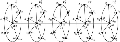
Example 2.6

The three cases of Theorem 2.5 are illustrated in Figs. 1–3.

Fig. 1 The ordering vertices of $P_4\odot C_6$ and the radio coloring of $P_4\odot C_6$ given in Case 1 of Theorem 2.5.

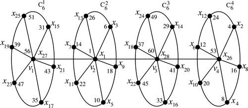
Fig. 2 The ordering vertices of $P_5\odot C_6$ and the radio coloring of $P_5\odot C_6$ given in Case 2 of Theorem 2.5.

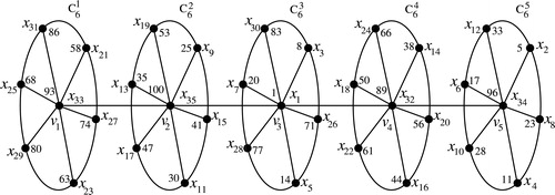
Fig. 3 The ordering vertices of $P_5\odot C_5$ and the radio coloring of $P_5\odot C_5$ given in Case 3 of Theorem 2.5.

Theorem 2.7

If $n=2p$ and $m\ge 5$ , then $rn(P_n\odot C_m)=(2m+2)p^2+2p$ .

Proof

To show $rn(P_n\odot C_m)\ge (2m+2)p^2+2p$, we use Theorem 2.4. Let $v_1{v}_2{v}_3\dots v_n$ be the path $P_n$. We choose $L_0=\{v_p,v_{p+1}\}$. Then we get, $\left|L_i\right|=2m+2$, for $1\le i\le p-1$, $\left|L_p\right|=2m$ and $\left|D_{2p+1}\right|=\left|V(P_n\odot C_m)\right|=mn+n$. Now, by Theorem 2.4, we have $$rn\left(G\right)\ge mn+n-2p+2\left(2p\right)+2\sum _{i=1}^{p-1}(2m+2)(p-i)+2\left(2m\right)\left(0\right)=(2m+2)p^2+2p.$$ Therefore, $rn(P_n\odot C_m)\ge (2m+2)p^2+2p$. ■

Theorem 2.8

If $n=2p+1$ and $m\ge 5$ , then $rn(P_n\odot C_m)\ge (2m+2)p^2+(2m+4)p+m+2$ .

Proof

Let $v_1{v}_2{v}_3\dots v_n$ be the path $P_n$. By choosing $L_0=\left\{v_{p+1}\right\}$ and using Theorem 2.4, we get the required lower bound. ■

In the remaining part of the paper, we determine the radio number of $P_n\odot P_m$ when $n$ is even. For $n$ odd, we give upper and lower bounds for the same. It is easy to see that $P_n\odot P_m$ is a subgraph of $P_n\odot C_m$.

Theorem 2.9

If $n=2p$ and $m\ge 4$ , then $rn(P_n\odot P_m)=(2m+2)p^2+2p$ .

Proof

Since $P_n\odot P_m$ is a subgraph of $P_n\odot C_m$, by Theorem 2.5, we have $rn(P_n\odot P_m)\le (2m+2)p^2+2p$ for $m\ge 5$. For $m=4$, we do exactly same as in Case 1 of Theorem 2.5 and get $rn(P_n\odot P_4)\le 10p^2+2p$. Now, to get the lower bound for $rn(P_n\odot P_m)$, we choose $L_0$ same as in the proof of Theorem 2.7 and we get $rn(P_n\odot P_m)\ge (2m+2)p^2+2p$. ■

Following theorem gives upper and lower bounds for $rn(P_n\odot P_m)$ when $n$ is odd.

Theorem 2.10

If $n=2p+1$ and $m\ge 4$ , then $$rn(P_n\odot P_m)\le \left\{\begin{array}{cc}(2m+2)p^2+(2m+4)p+m+2+(\frac{m}{2}-1)p\hfill & ifmiseven,\hfill \\ (2m+2)p^2+(2m+4)p+m+2+\left(\frac{m-1}{2}\right)p\hfill & ifmisodd,\hfill \end{array}\right.$$ and $rn(P_n\odot P_m)\ge (2m+2)p^2+(2m+4)p+m+2$ .

Proof

Since $P_n\odot P_m$ is a subgraph of $P_n\odot C_m$, by Theorem 2.5, we have $rn(P_n\odot P_m)\le (2m+2)p^2+(2m+4)p+m+2+(\frac{m}{2}-1)p$ if $m\ge 6$ is even and $rn(P_n\odot P_m)\le (2m+2)p^2+(2m+4)p+m+2+\left(\frac{m-1}{2}\right)p$ if $m\ge 5$ is odd. For $m=4$, we do exactly same as in Case 2 of Theorem 2.5 and get $rn(P_n\odot P_4)\le 10p^2+13p+6$. Now, to get the lower bound for $rn(P_n\odot P_m)$, we choose $L_0$ same as in the proof of Theorem 2.8 and obtain $rn(P_n\odot P_m)\ge (2m+2)p^2+(2m+4)p+m+2$. ■

References

- HaleWilliam K., Frequency assignment: Theory and applications Proc. IEEE 68 12 1980 1497–1514
- ChartrandGrayErwinDavidHararyFrankZhangPhing, Radio labelings of graphs Bull. Inst. Combin. Appl. 332001 77–85
- KchikechMustaphaKhennoufaRiadhTogniOlivier, Radio k-labelings for cartesian products of graphs Discuss. Math. Graph Theory 28 1 2008 165–178
- KimByeong MoonHwangWoonjaeSongByung Chul, Radio number for the product of a path and a complete graph J. Comb. Optim. 30 1 2015 139–149
- AjayiDeborah OlayideAdefokunTayo Charles, On bounds of radio number of certain product graphs J. Nigerian Math. Soc. 37 2 2018 71–76
- Morris-RiveraMarcTomovaMaggyWyelsCindyYeagerAaron, The radio number of Cn□Cn Ars Combin. 1202015 7–21
- SahaLaxmanPanigrahiPratima, On the radio number of toroidal grids Australas. J. Combin. 552013 273–288
- KolaSrinivasa RaoPanigrahiPratima, A lower bound for radio k-chromatic number of an arbitrary graph Contrib. Discrete Math. 10 2 2015
- DasSandipGhoshSasthi C.NandiSoumenSenSagnik, A lower bound technique for radio k-coloring Discrete Math. 340 5 2017 855–861