Numerical computation of fractional Black–Scholes equation arising in financial market

Peer review under responsibility of Mansoura University.

Abstract

The aim of present paper is to present a numerical algorithm for time-fractional Black–Scholes equation with boundary condition for a European option problem by using homotopy perturbation method and homotopy analysis method. The fractional derivative is described in the Caputo sense. The methods give an analytic solution in the form of a convergent series with easily computable components, requiring no linearization or small perturbation. The methods show improvements over existing analytical techniques. Two examples are given and show that the homotopy perturbation method and homotopy analysis method are very effective and convenient overcomes the difficulty of traditional methods. The numerical results show that the approaches are easy to implement and accurate when applied to time-fractional Black–Scholes equation.

Keywords:

• Black–Scholes equation
• European option pricing
• Fractional derivatives
• Analytical solution
• Homotopy perturbation method
• Homotopy analysis method
• Mathematics Subject Classification
• 2010
• 34A08
• 35A20

1 Introduction

In 1973, Fischer Black and Myron Scholes [1] derived the famous theoretical valuation formula for options. The main conceptual idea of Black and Scholes lie in the construction of a riskless portfolio taking positions in bonds (cash), option and the underlying stock. Such an approach strengthens the use of the no-arbitrage principle as well. Thus, the Black–Scholes formula is used as a model for valuing European (the option can be exercised only on a specified future date) or American (the option can be exercised at any time up to the date, the option expires) call and put options on a non-dividend paying stock [2]. Derivation of a closed form solution to the Black–Scholes equation depends on the fundamental solution of the heat equation. Hence, it is important, at this point, to transform the Black–Scholes equation to the heat equation by change of variables. Having found the closed form solution to the heat equation, it is possible to transform it back to find the corresponding solution of the Black–Scholes PDE. Financial models were generally formulated in terms of stochastic differential equations. However, it was soon found that under certain restrictions these models could written as linear evolutionary PDEs with variable coefficients [3]. Thus, the Black–Scholes model for the value of an option is described by the equation (1) $\frac{\partial v}{\partial t}+\frac{{\sigma }^2{x}^2}{2}\frac{{\partial }^{2}v}{\partial x^2}+r\left(t\right)x\frac{\partial v}{\partial x}-r\left(t\right)v=0,(x,t)\in R^{+}\times (0,T)$(1) where v(x,t) is the European call option price at asset price x and at time t, K is the exercise price, T is the maturity, r(t) is the risk free interest rate, and σ(x,t) represents the volatility function of underlying asset. Let us denote by v_c(x,t) and v_p(x,t) the value of the European call and put options, respectively. Then, the payoff functions are (2) $v_c(x,t)=\max (x-E,0),v_p(x,t)=\max (E-x,0),$(2) where E denotes the expiration price for the option and the function max(x,0) gives the larger value between x and 0. During the past few decades, many researchers studied the existence of solutions of the Black-Scholes model using many methods in [4^{[5][6][7][8][9][10][11]}–12]. Many important phenomena are well described by fractional differential equations in electromagnetics, acoustics, viscoelasticity, electro chemistry and material science. That is because of the fact that, a realistic modelling of a physical phenomenon having dependence not only at the time instant, but also the previous time history can be successfully achieved by using fractional calculus. The book by Oldham and Spanier [13] has played a key role in the development of the subject. Some fundamental results related to solving fractional differential equations may be found in Miller and Rose [14], Podlubny [15], Kilbas et al. [16], Podlubny [17].

The objective of this paper is to extend the application of homotopy perturbation method (HPM) and homotopy analysis method (HAM) to obtain analytic and approximate solution fractional Black–Scholes equations. The homotopy perturbation method is first proposed and applied by Chinese mathematician He [18^[19][20][21]–22]. The method was successfully applied to space–time fractional advection–dispersion equation by Yildirim and Kocak [23], fractional Zakharov–Kuznetsov equations by Yildirim and Gulkanat [24], fractional modified Kdv equation by Abdulaziz et al. [25], Fractional Chemical Engineering equation by Khan et al. [26]. One of the highly applicable analytical techniques is homotopy analysis method (HAM), which was introduced and developed by Liao [27^[28][29][30]–31]. This method is applied to solve many nonlinear problems [32^[33][34]–35] and the references therein to handle a wide variety of scientific and engineering applications: linear and nonlinear as well as homogeneous and inhomogeneous.

The fractional Black–Scholes equation can be written as (3) $D_t^{\alpha }v+\frac{{\sigma }^2{x}^2}{2}{D}_x^{2}v+r\left(t\right)x{D}_{x}v-r\left(t\right)v=0,0<\alpha \le 1,$(3) equipped with the terminal and boundary condition (4) $v(x,T)=\max (x-E,0),x\in R^{+},v(0,t)=0,t\in [0,T]$(4)

2 Basic definitions of fractional calculus

In this section, we mention the following basic definitions of fractional calculus which are used further in the present paper.

Definition 1

The Riemann-Liouville fractional integral operator of order α > 0, of a function $f\left(t\right)\in C_{\mu },\mu \ge \mathrm{-}1$ is defined as [15]: (5) $J^{\alpha }f\left(t\right)=\frac{1}{\Gamma \left(\alpha \right)}\underset{0}{\overset{t}{\int }}{(t-\tau )}^{\alpha -1}f\left(\tau \right)d\tau ,(\alpha >0),$(5) (6) $J^{0}f\left(t\right)=f\left(t\right)\text{.}$(6)

For the Riemann-Liouville fractional integral we have: (7) $J^{\alpha }{t}^{\gamma }=\frac{\Gamma (\gamma +1)}{\Gamma (\gamma +\alpha +1)}{t}^{\alpha +\gamma }\text{.}$(7)

Definition 2

The fractional derivative of f(t) in the Caputo sense is defined as [36]: (8) $D_t^{\alpha }f\left(t\right)=J^{m-\alpha }{D}^{n}f\left(t\right)=\frac{1}{\Gamma (n-\alpha )}\underset{0}{\overset{t}{\int }}{(t-\tau )}^{m-\alpha -1}{f}^{\left(m\right)}\left(\tau \right)d\tau ,$(8) for $m\mathrm{-}1\mathrm{<}\alpha \le m,m\in N,t\mathrm{>}0$.

For the Riemann-Liouville fractional integral and the Caputo fractional derivative, we have the following relation (9) $J_t^{\alpha }{D}_t^{\alpha }f\left(t\right)=f\left(t\right)-\sum _{k=0}^{m-1}{f}^{\left(k\right)}(0+)\frac{t^k}{k!}\text{.}$(9)

Definition 3

The Mittag-Leffler is defined as [37]: (10) $E_{\alpha }\left(z\right)=\sum _{k=0}^{\infty }\frac{z^k}{\Gamma \left(\alpha k+1\right)},\left(\alpha \in C,\mathrm{Re}\left(\alpha \right)>0\right)\text{.}$(10)

3 Basic idea of homotopy perturbation method (HPM)

To illustrate the basic idea of the HPM for fractional differential equations, we consider the following problem (11) $D_{\ast t}^{\alpha }u(x,t)=v(x,t)-Lu(x,t)-Nu(x,t),m-1<\alpha \le m,m\in N,t\ge 0,x\in R^n$(11)

Subject to the initial and boundary conditions (12) $u^{\left(i\right)}\left(\mathrm{0,0}\right)=c_i,B\left(u,\frac{\partial u}{\partial x_j},\frac{\partial u}{\partial t}\right)=0,i=\mathrm{0,1,2},\dots ,m-1,j=\mathrm{1,2,3},\dots ,n$(12) where L is a linear operator, while N is a nonlinear operator, v is a known analytical function and $D_{\ast t}^{\alpha }$ denotes the fractional derivative in the Caputo sense [15]. u is assumed to be a causal function of time, i.e., vanishing for t < 0. Also u⁽ⁱ⁾(x,t) is the ith derivative of u, c_i, i = 0,1,2,…,m−1 are the specified initial conditions and B is a boundary operator.

We construct the following homotopy (13) $(1-p)D_{\ast t}^{\alpha }u(x,t)+p\left(D_{\ast t}^{\alpha }u(x,t)+Lu(x,t)+Nu(x,t)-v(x,t)\right)=0,p\in \left[\mathrm{0,1}\right]$(13) which is equivalent to (14) $D_{\ast t}^{\alpha }u(x,t)+p\left(Lu(x,t)+Nu(x,t)-v(x,t)\right)=0,p\in \left[\mathrm{0,1}\right]$(14)

The homotopy parameter p always changes from zero to unity. In case p = 0, Eq. (14)(14) $D_{\ast t}^{\alpha }u(x,t)+p\left(Lu(x,t)+Nu(x,t)-v(x,t)\right)=0,p\in \left[\mathrm{0,1}\right]$(14) becomes (15) $D_{\ast t}^{\alpha }u(x,t)=0,$(15) when p = 1, Eq. (14)(14) $D_{\ast t}^{\alpha }u(x,t)+p\left(Lu(x,t)+Nu(x,t)-v(x,t)\right)=0,p\in \left[\mathrm{0,1}\right]$(14) turns out to be the original fractional differential equation. The homotopy parameter p is used to expand the solution in the following form (16) $u(x,t)=u_0(x,t)+p{u}_1(x,t)+p^2{u}_2(x,t)+p^3{u}_3(x,t)+\dots \text{.}$(16)

For nonlinear problems, we set Nu(x,t) = S(x,t). Substituting Eq. (16)(16) $u(x,t)=u_0(x,t)+p{u}_1(x,t)+p^2{u}_2(x,t)+p^3{u}_3(x,t)+\dots \text{.}$(16) into Eq. (14)(14) $D_{\ast t}^{\alpha }u(x,t)+p\left(Lu(x,t)+Nu(x,t)-v(x,t)\right)=0,p\in \left[\mathrm{0,1}\right]$(14) and equating the terms with identical power of p, we obtain a sequence of equations of the form (17) $\begin{array}{l}{p}^0:D_{\ast t}^{\alpha }{u}_0(x,t)=0,\\ p^1:D_{\ast t}^{\alpha }{u}_1(x,t)=-L{u}_0(x,t)-S_0\left(u_0\right(x,t\left)\right)+v(x,t),\\ p^2:D_{\ast t}^{\alpha }{u}_2(x,t)=-L{u}_1(x,t)-S_1\left(u_0\right(x,t),u_1(x,t\left)\right),\\ p^j:D_{\ast t}^{\alpha }{u}_j(x,t)=-L{u}_{j-1}(x,t)-S_{j-1}\left(u_0\right(x,t),u_1(x,t),u_2(x,t),\dots ,u_{j-1}(x,t\left)\right),j=\mathrm{2,3,4},\dots \end{array}$(17)

The functions S₀,S₁,S₂,… satisfy the following equation (18) $S\left(u_0(x,t)+p{u}_1(x,t)+p^2{u}_2(x,t)+p^3{u}_3(x,t)+\dots \right)=S_0\left(u_0(x,t)\right)+p{S}_1\left(u_0(x,t),u_1(x,t)\right)+p^2{S}_2\left(u_0(x,t),u_1(x,t),u_2(x,t)\right)+\dots \text{.}$(18)

Applying the inverse operator$J_t^{\alpha }$ on both sides of the equation (15)(15) $D_{\ast t}^{\alpha }u(x,t)=0,$(15) and considering the initial and boundary conditions, the various components of the series solution are given by (19) $\begin{array}{l}{u}_0(x,t)=\sum _{i=0}^{n-1}{c}_i\frac{t^i}{i!},\\ u_1(x,t)=-J_t^{\alpha }\left(L{u}_0\right(x,t\left)\right)-J_t^{\alpha }{S}_0\left(u_0\right(x,t\left)\right)+J_t^{\alpha }v(x,t),\\ u_j(x,t)=-J_t^{\alpha }\left(L{u}_{j-1}\right(x,t\left)\right)-J_t^{\alpha }{S}_{j-1}\left(u_0\right(x,t),u_1(x,t),u_2(x,t),\dots ,u_{j-1}(x,t\left)\right),j=\mathrm{2,3,4},\mathrm{...}\text{.}\end{array}$(19)

Hence, the HPM solution u(x,t) is given by (20) $u(x,t)=\sum _{i=0}^{\infty }{u}_i(x,t)$(20)

4 Basic idea of homotopy analysis method (HAM)

In order to show the basic idea of HAM, consider the following nonlinear fractional differential equation (21) $N_F\left[u\right(x,t\left)\right]=0,$(21) where N_F is a nonlinear fractional operator, x and t denote the independent variables and u is an unknown function. For simplicity, we ignore all boundary or initial conditions, which can be treated in the similar way. By means of the HAM, we first construct the so-called zeroth-order deformation equation as (22) $(1-q)L_F\left[\varphi \right(x,t;q)-u_0(x,t\left)\right]=\hslash qH(x,t)N_F\left[u\right(x,t\left)\right],$(22) where $q\in \left[\mathrm{0,1}\right]$ is the embedding parameter, ℏ ≠ 0 is an auxiliary parameter, L_F is an auxiliary linear operator, φ(x,t ;q) is an unknown function,u₀(x,t) is an initial guess of u(x,t) and H(x,t) denotes a nonzero auxiliary function. Obviously, when the embedding parameter q = 0 and q = 1, it holds (23) $\varphi (x,t;0)=u_0(x,t),\varphi (x,t;1)=u(x,t),$(23) respectively. Thus as q increases from 0 to 1, the solution φ(x,t ;q) varies from the initial guess u₀(x,t) to the solution u(x,t). Expanding φ(x,t ;q) in Taylor series with respect to q, we have (24) $\varphi (x,t;q)=u_0(x,t)+\sum _{m=1}^{\infty }{u}_m(x,t)q^m,$(24) where (25) $u_m(x,t)=\frac{1}{m!}{\frac{{\partial }^m\varphi (x,t;q)}{\partial q^m}|}_{q=0}\text{.}$(25)

If the auxiliary linear operator, the initial guess, the auxiliary parameter ℏ, and the auxiliary function are properly chosen, the series (24)(24) $\varphi (x,t;q)=u_0(x,t)+\sum _{m=1}^{\infty }{u}_m(x,t)q^m,$(24) converges at q = 1, then we have (26) $u(x,t)=u_0(x,t)+\sum _{m=1}^{\infty }{u}_m(x,t),$(26) which must be one of the solutions of the original nonlinear fractional differential equations. According to the definition (26)(26) $u(x,t)=u_0(x,t)+\sum _{m=1}^{\infty }{u}_m(x,t),$(26) , the governing equation can be deduced from the zero-order deformation (22)(22) $(1-q)L_F\left[\varphi \right(x,t;q)-u_0(x,t\left)\right]=\hslash qH(x,t)N_F\left[u\right(x,t\left)\right],$(22) . Define the vectors (27) ${\overrightarrow{u}}_m=\left\{u_0\right(x,t),u_1(x,t),\dots ,u_m(x,t\left)\right\}\text{.}$(27)

Differentiating the zeroth-order deformation Eq. (22)(22) $(1-q)L_F\left[\varphi \right(x,t;q)-u_0(x,t\left)\right]=\hslash qH(x,t)N_F\left[u\right(x,t\left)\right],$(22) m-times with respect to q and then dividing them by m! and finally setting q = 0, we get the following mth-order deformation equation: (28) $L_F\left[u_m\right(x,t)-{\chi }_m{u}_{m-1}(x,t\left)\right]=\hslash H(x,t){\Re }_m\left({\overrightarrow{u}}_{m-1}\right),$(28) where (29) ${\Re }_m\left({\overrightarrow{u}}_{m-1}\right)=\frac{1}{(m-1)!}{\frac{{\partial }^{m-1}{N}_F\left[\varphi \right(x,t;q\left)\right]}{\partial q^{m-1}}|}_{q=0},$(29) and (30) ${\chi }_m=\{\begin{array}{l}0,m\le 1,\\ 1,m>1.\end{array}$(30)

5 Numerical examples of European option pricing equation

In order to illustrate the advantages and the accuracy of the HPM and HAM for solving fractional Black-Scholes equation with boundary condition for a European option problem, we have applied the methods for two different examples.

Example 1

We consider the fractional Black–Scholes equation as [12] (31) $\frac{{\partial }^{\alpha }v}{\partial t^{\alpha }}=\frac{{\partial }^{2}v}{\partial x^2}+(k-1)\frac{\partial v}{\partial x}-kv,0<\alpha \le 1,$(31) with initial condition v(x,0) = max (e^x−1, 0). Notice that this system of equations contains just two dimensionless parameters k = 2 r/σ², where k represents the balance between the rate of interests and the variability of stock returns and the dimensionless time to expiry ½σ²T, even though there are four dimensional parameters, E, T, σ² and r, in the original statements of the problem.

According to the HPM [18^[19][20][21]–22], we construct the following homotopy (32) $D_t^{\alpha }v-p\left(D_x^{2}v+(k-1)D_{x}v-kv\right)=0,$(32) where the homotopy parameter p is considered as a small parameter $p\in \left[\mathrm{0,1}\right]$. Now applying the classical perturbation technique, we can assume that the solution of Eq. (32)(32) $D_t^{\alpha }v-p\left(D_x^{2}v+(k-1)D_{x}v-kv\right)=0,$(32) can be expressed as power series in p as given below (33) $v=v_0+p{v}_1+p^2{v}_2+p^3{v}_2+\dots$(33)

Substituting (33)(33) $v=v_0+p{v}_1+p^2{v}_2+p^3{v}_2+\dots$(33) into (32)(32) $D_t^{\alpha }v-p\left(D_x^{2}v+(k-1)D_{x}v-kv\right)=0,$(32) and equating the coefficients of like powers of p, we get the following set of differential equations that (34) $p^0:D_t^{\alpha }{v}_0(x,t)=0,$(34) (35) $p^n:D_t^{\alpha }{v}_n(x,t)=D_x^2{v}_{n-1}(x,t)+(k-1)D_x{v}_{n-1}(x,t)-k{v}_{n-1}(x,t),n\ge 1\text{.}$(35)

The above equations can be easily solved by applying the operator $J_t^{\alpha }$ to (34(34) $p^0:D_t^{\alpha }{v}_0(x,t)=0,$(34) ,35(35) $p^n:D_t^{\alpha }{v}_n(x,t)=D_x^2{v}_{n-1}(x,t)+(k-1)D_x{v}_{n-1}(x,t)-k{v}_{n-1}(x,t),n\ge 1\text{.}$(35) ) giving the various components v_n(x,t) as $\begin{array}{l}{v}_0(x,t)=v(x,0)=\max (e^x-\mathrm{1,0}),\\ v_1(x,t)=-\max (e^x,0)\frac{(-k{t}^{\alpha })}{\Gamma (\alpha +1)}+\max (e^x-\mathrm{1,0})\frac{(-k{t}^{\alpha })}{\Gamma (\alpha +1)},\\ v_2(x,t)=-\max (e^x,0)\frac{{(-k{t}^{\alpha })}^2}{\Gamma (2\alpha +1)}+\max (e^x-\mathrm{1,0})\frac{{(-k{t}^{\alpha })}^2}{\Gamma (2\alpha +1)},\\ ⋮\end{array}$

Finally, we approximate the analytical solution v(x,t) by the series $v(x,t)=\underset{N\to \infty }{\lim }\sum _{n=0}^{N-1}{v}_n(x,t),$ then we get $v(x,t)=\max (e^x,0)-\max (e^x,0)\left(1+\frac{(-k{t}^{\alpha })}{\Gamma (\alpha +1)}+\frac{{(-k{t}^{\alpha })}^2}{\Gamma (2\alpha +1)}+\cdots \right)+\max (e^x-\mathrm{1,0})\left(1+\frac{(-k{t}^{\alpha })}{\Gamma (\alpha +1)}+\frac{{(-k{t}^{\alpha })}^2}{\Gamma (2\alpha +1)}+\cdots \right)$ or $v(x,t)=\max (e^x,0)-\max (e^x,0)\sum _{n=0}^{\infty }\frac{{(-k{t}^{\alpha })}^n}{\Gamma (n\alpha +1)}+\max (e^x-\mathrm{1,0})\sum _{n=0}^{\infty }\frac{{(-k{t}^{\alpha })}^n}{\Gamma (n\alpha +1)},$ and in closed form (36) $v(x,t)=\max (e^x,0)\left(1-E_{\alpha }(-k{t}^{\alpha })\right)+\max (e^x-\mathrm{1,0})E_{\alpha }(-k{t}^{\alpha })\text{.}$(36)

This is the exact solution of the given problem of (31)(31) $\frac{{\partial }^{\alpha }v}{\partial t^{\alpha }}=\frac{{\partial }^{2}v}{\partial x^2}+(k-1)\frac{\partial v}{\partial x}-kv,0<\alpha \le 1,$(31) .

To solve the Eq. (31)(31) $\frac{{\partial }^{\alpha }v}{\partial t^{\alpha }}=\frac{{\partial }^{2}v}{\partial x^2}+(k-1)\frac{\partial v}{\partial x}-kv,0<\alpha \le 1,$(31) by HAM, we choose the auxiliary operators as follows $L_F\left[\varphi \right(x,t;q\left)\right]=D_t^{\alpha }\left[\varphi \right(x,t;q\left)\right],$ with the property L_F[c₁] = 0.

Using the above definition, we first construct the zeroth-order deformation equations as (37) $(1-q)L_F\left[\varphi \right(x,t;q)-{\chi }_m{v}_0(x,t\left)\right]=\hslash q{N}_F\left[\varphi \right(x,t;q\left)\right]\text{.}$(37)

Obviously, when the embedding parameter q = 0 and q = 1, it holds (38) $\varphi (x,t;0)=v_0(x,t),\varphi (x,t;1)=v(x,t)\text{.}$(38)

Differentiating the zeroth-order deformation Eq. (37)(37) $(1-q)L_F\left[\varphi \right(x,t;q)-{\chi }_m{v}_0(x,t\left)\right]=\hslash q{N}_F\left[\varphi \right(x,t;q\left)\right]\text{.}$(37) m-times with respect to q and then dividing them by m! and finally setting q = 0, we get the following mth-order deformation equations (39) $L_F\left[v_m\right(x,t)-{\chi }_m{v}_{m-1}(x,t\left)\right]=\hslash {\Re }_m\left({\overrightarrow{u}}_{m-1}\right),$(39) where (40) ${\Re }_m\left({\overrightarrow{v}}_{m-1}\right)=\frac{{\partial }^{\alpha }{v}_{m-1}}{\partial t^{\alpha }}-\frac{{\partial }^2{v}_{m-1}}{\partial x^2}-(k-1)\frac{\partial v_{m-1}}{\partial x}+k{v}_{m-1}\text{.}$(40)

On applying the operator $J_t^{\alpha }$ both the sides of Eq. (39)(39) $L_F\left[v_m\right(x,t)-{\chi }_m{v}_{m-1}(x,t\left)\right]=\hslash {\Re }_m\left({\overrightarrow{u}}_{m-1}\right),$(39) , we get (41) $v_m(x,t)={\chi }_m{v}_{m-1}(x,t)+\hslash {\Re }_m\left({\overrightarrow{u}}_{m-1}\right),$(41) subsequently solving the mth-order deformation equations one has $\begin{array}{l}{v}_0(x,t)=\max (e^x-\mathrm{1,0}),\\ v_1(x,t)=\hslash \max (e^x,0)\frac{(-k{t}^{\alpha })}{\Gamma (\alpha +1)}-\hslash \max (e^x-\mathrm{1,0})\frac{(-k{t}^{\alpha })}{\Gamma (\alpha +1)},\\ v_2(x,t)=\hslash (1+\hslash )\max (e^x,0)\frac{(-k{t}^{\alpha })}{\Gamma (\alpha +1)}-\hslash (1+\hslash )\max (e^x-\mathrm{1,0})\frac{(-k{t}^{\alpha })}{\Gamma (\alpha +1)}-{\hslash }^2\max (e^x,0)\frac{{(-k{t}^{\alpha })}^2}{\Gamma (2\alpha +1)}+{\hslash }^2\max (e^x-\mathrm{1,0})\frac{{(-k{t}^{\alpha })}^2}{\Gamma (2\alpha +1)},\end{array}$ and so on.

Therefore, the HAM series solution is (42) $v(x,t)=\max (e^x-\mathrm{1,0})+\hslash \max (e^x,0)\frac{(-k{t}^{\alpha })}{\Gamma (\alpha +1)}-\hslash \max (e^x-\mathrm{1,0})\frac{(-k{t}^{\alpha })}{\Gamma (\alpha +1)}+\hslash (1+\hslash )\max (e^x,0)\frac{(-k{t}^{\alpha })}{\Gamma (\alpha +1)}-\hslash (1+\hslash )\max (e^x-\mathrm{1,0})\frac{(-k{t}^{\alpha })}{\Gamma (\alpha +1)}-{\hslash }^2\max (e^x,0)\frac{{(-k{t}^{\alpha })}^2}{\Gamma (2\alpha +1)}+{\hslash }^2\max (e^x-\mathrm{1,0})\frac{{(-k{t}^{\alpha })}^2}{\Gamma (2\alpha +1)}+\dots$(42)

Taking ℏ = −1, we get the same solution as obtained by HPM.

Case 1

Consider the vanilla call option with parameter [5]

σ = 0.2, r = 0.04, α = 1, τ = 0.5 years then k = 2.

In this case, we get the solution of Eq. (31)(31) $\frac{{\partial }^{\alpha }v}{\partial t^{\alpha }}=\frac{{\partial }^{2}v}{\partial x^2}+(k-1)\frac{\partial v}{\partial x}-kv,0<\alpha \le 1,$(31) (43) $v(x,t)=\max (e^x,0)\left(1-e^{-2t}\right)+\max (e^x-\mathrm{1,0})e^{-2t}\text{.}$(43)

This is the given exact solution of the standard Black–Scholes equation.

Case 2

In this case, we consider the vanilla call option with parameter [5]

σ = 0.2, r = 0.01, α = 1, τ = 1 year then k = 5.

We get the solution of Eq. (31)(31) $\frac{{\partial }^{\alpha }v}{\partial t^{\alpha }}=\frac{{\partial }^{2}v}{\partial x^2}+(k-1)\frac{\partial v}{\partial x}-kv,0<\alpha \le 1,$(31) (44) $v(x,t)=\max (e^x,0)\left(1-e^{-5t}\right)+\max (e^x-\mathrm{1,0})e^{-5t}\text{.}$(44)

This is the exact solution for the given case.

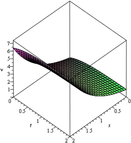
The numerical results for the fractional Black–Scholes Eq. (31)(31) $\frac{{\partial }^{\alpha }v}{\partial t^{\alpha }}=\frac{{\partial }^{2}v}{\partial x^2}+(k-1)\frac{\partial v}{\partial x}-kv,0<\alpha \le 1,$(31) obtained by using the HPM and HAM for various values of x and t, when α = 1 and k = 2 are shown by Fig. 1. It can be observed from Fig. 1 that ν(x,t) increases with the increase in both x and t.

Fig. 1 The surface shows the v(x, t) for (31(31) $\frac{{\partial }^{\alpha }v}{\partial t^{\alpha }}=\frac{{\partial }^{2}v}{\partial x^2}+(k-1)\frac{\partial v}{\partial x}-kv,0<\alpha \le 1,$(31) ) with respect to x and t, when α = 1 and k = 2.

Examples 2

In this example, we consider the following generalized Black–Scholes equation as [6] (45) $\frac{{\partial }^{\alpha }v}{\partial t^{\alpha }}+0.08{(2+\sin x)}^2{x}^2\frac{{\partial }^{2}v}{\partial x^2}+0.06x\frac{\partial v}{\partial x}-0.06v=0,0<\alpha \le 1,$(45) with initial condition v(x,0) = max (x−25 e^−0.06, 0).

We construct the homotopy which satisfies the relation (46) $D_t^{\alpha }v+p[0.08{(2+\sin x)}^2{x}^2{D}_x^{2}v+0.06x{D}_{x}v-0.06v]=0,p\in \left[\mathrm{0,1}\right]\text{.}$(46)

Substituting (33)(33) $v=v_0+p{v}_1+p^2{v}_2+p^3{v}_2+\dots$(33) into (46)(46) $D_t^{\alpha }v+p[0.08{(2+\sin x)}^2{x}^2{D}_x^{2}v+0.06x{D}_{x}v-0.06v]=0,p\in \left[\mathrm{0,1}\right]\text{.}$(46) and equating the coefficients of like powers of p, we get following set of differential equations (47) $p^0:D_t^{\alpha }{v}_0(x,t)=0,$(47) (48) $p^n:D_t^{\alpha }{v}_n(x,t)=-\left(0.08{(2+\sin x)}^2{x}^2{D}_x^2{v}_{n-1}(x,t)+0.06x{D}_x{v}_{n-1}(x,t)-0.06v_{n-1}(x,t)\right),n\ge 1\text{.}$(48)

Consequently, the above system of nonlinear equations can be easily solved by applying the operator $J_t^{\alpha }$ to (47(47) $p^0:D_t^{\alpha }{v}_0(x,t)=0,$(47) ,48(48) $p^n:D_t^{\alpha }{v}_n(x,t)=-\left(0.08{(2+\sin x)}^2{x}^2{D}_x^2{v}_{n-1}(x,t)+0.06x{D}_x{v}_{n-1}(x,t)-0.06v_{n-1}(x,t)\right),n\ge 1\text{.}$(48) ) giving the various components v_n(x,t), thus enabling the series solution to be entirely determined. The first few components of the homotopy perturbation solution for Eq. (45)(45) $\frac{{\partial }^{\alpha }v}{\partial t^{\alpha }}+0.08{(2+\sin x)}^2{x}^2\frac{{\partial }^{2}v}{\partial x^2}+0.06x\frac{\partial v}{\partial x}-0.06v=0,0<\alpha \le 1,$(45) are derived as follows: $\begin{array}{l}{v}_0(x,t)=v(x,0)=\max (x-25e^{-0.06},0),\\ v_1(x,t)=-\frac{x\left(0.06t^{\alpha }\right)}{\Gamma (\alpha +1)}+\max (x-25e^{-0.06},0)\frac{\left(0.06t^{\alpha }\right)}{\Gamma (\alpha +1)},\\ v_2(x,t)=-\frac{x{\left(0.06t^{\alpha }\right)}^2}{\Gamma (2\alpha +1)}+\max (x-25e^{-0.06},0)\frac{{\left(0.06t^{\alpha }\right)}^2}{\Gamma (2\alpha +1)},\\ ⋮\end{array}$ and so on.

Finally, we approximate the analytical solution v(x,t) by the series $v(x,t)=\underset{N\to \infty }{\lim }{v}_N(x,t),$ where $v_N(x,t)=\sum _{n=0}^{N-1}{v}_n(x,t),$ then we get (49) $v(x,t)=x(1-E_{\alpha }(0.06t^{\alpha }\left)\right)+\max (x-25e^{-0.06},0)E_{\alpha }\left(0.06t^{\alpha }\right)\text{.}$(49) which is analytical solution of the fractional Black-Scholes Eq. (45)(45) $\frac{{\partial }^{\alpha }v}{\partial t^{\alpha }}+0.08{(2+\sin x)}^2{x}^2\frac{{\partial }^{2}v}{\partial x^2}+0.06x\frac{\partial v}{\partial x}-0.06v=0,0<\alpha \le 1,$(45) .

To solve the Eq. (45)(45) $\frac{{\partial }^{\alpha }v}{\partial t^{\alpha }}+0.08{(2+\sin x)}^2{x}^2\frac{{\partial }^{2}v}{\partial x^2}+0.06x\frac{\partial v}{\partial x}-0.06v=0,0<\alpha \le 1,$(45) by HAM, we choose the auxiliary operators as follows $L_F\left[\varphi \right(x,t;q\left)\right]=D_t^{\alpha }\left[\varphi \right(x,t;q\left)\right],$ with the property L_F [c₁] = 0.

Using the above definition, we first construct the zeroth-order deformation equations as (50) $(1-q)L_F\left[\varphi \right(x,t;q)-{\chi }_m{v}_0(x,t\left)\right]=\hslash q{N}_F\left[\varphi \right(x,t;q\left)\right]\text{.}$(50)

Obviously, when the embedding parameter q = 0 and q = 1, it holds (51) $\varphi (x,t;0)=v_0(x,t),\varphi (x,t;1)=v(x,t)\text{.}$(51)

Differentiating the zeroth-order deformation Eq. (50)(50) $(1-q)L_F\left[\varphi \right(x,t;q)-{\chi }_m{v}_0(x,t\left)\right]=\hslash q{N}_F\left[\varphi \right(x,t;q\left)\right]\text{.}$(50) m-times with respect to q and then dividing them by m! and finally setting q = 0, we get the following mth-order deformation equations (52) $L_F\left[v_m\right(x,t)-{\chi }_m{v}_{m-1}(x,t\left)\right]=\hslash {\Re }_m\left({\overrightarrow{u}}_{m-1}\right),$(52) where (53) ${\Re }_m\left({\overrightarrow{u}}_{m-1}\right)=\frac{{\partial }^{\alpha }{v}_{m-1}}{\partial t^{\alpha }}+0.08{(2+\sin x)}^2{x}^2\frac{{\partial }^2{v}_{m-1}}{\partial x^2}+0.06x\frac{\partial v_{m-1}}{\partial x}-0.06v_{m-1}\text{.}$(53)

On applying the operator $J_t^{\alpha }$ both the sides of Eq. (52)(52) $L_F\left[v_m\right(x,t)-{\chi }_m{v}_{m-1}(x,t\left)\right]=\hslash {\Re }_m\left({\overrightarrow{u}}_{m-1}\right),$(52) , we get (54) $v_m(x,t)={\chi }_m{v}_{m-1}(x,t)+\hslash {\Re }_m\left({\overrightarrow{u}}_{m-1}\right),$(54) subsequently solving the mth-order deformation equations one has $\begin{array}{l}{v}_0(x,t)=\max (x-25e^{-0.06},0),\\ v_1(x,t)=\hslash x\frac{\left(0.06t^{\alpha }\right)}{\Gamma (\alpha +1)}-\hslash \max (x-25e^{-0.06},0)\frac{\left(0.06t^{\alpha }\right)}{\Gamma (\alpha +1)},\\ v_2(x,t)=\hslash (1+\hslash )x\frac{\left(0.06t^{\alpha }\right)}{\Gamma (\alpha +1)}-\hslash (1+\hslash )\max (x-25e^{-0.06},0)\frac{\left(0.06t^{\alpha }\right)}{\Gamma (\alpha +1)}-{\hslash }^{2}x\frac{{\left(0.06t^{\alpha }\right)}^2}{\Gamma (2\alpha +1)}+{\hslash }^2\max (x-25e^{-0.06},0)\frac{{\left(0.06t^{\alpha }\right)}^2}{\Gamma (2\alpha +1)},\\ ⋮\end{array}$ and so on.

Therefore, the HAM series solution is (55) $v(x,t)=\max (x-25e^{-0.06},0)+\hslash x\frac{\left(0.06t^{\alpha }\right)}{\Gamma (\alpha +1)}-\hslash \max (x-25e^{-0.06},0)\frac{\left(0.06t^{\alpha }\right)}{\Gamma (\alpha +1)}+\hslash (1+\hslash )x\frac{\left(0.06t^{\alpha }\right)}{\Gamma (\alpha +1)}-\hslash (1+\hslash )\max (x-25e^{-0.06},0)\frac{\left(0.06t^{\alpha }\right)}{\Gamma (\alpha +1)}-{\hslash }^{2}x\frac{{\left(0.06t^{\alpha }\right)}^2}{\Gamma (2\alpha +1)}+{\hslash }^2\max (x-25e^{-0.06},0)\frac{{\left(0.06t^{\alpha }\right)}^2}{\Gamma (2\alpha +1)}+\cdots \text{.}$(55)

Taking ℏ = −1, we get the same solution as obtained by HPM.

6 Concluding remarks

In this study, the HPM and HAM are implemented to solve the time-fractional Black–Scholes equation with boundary condition for a European option problem. They provide the solutions in terms of convergent series with easily computable components in a direct way without using linearization, perturbation or restrictive assumptions. The solution obtained with the help of HAM is more general as compared to HPM solution. We can easily recover all results HPM by assuming ℏ = −1. The results show that the HPM and HAM are powerful and efficient techniques in finding exact and approximate solutions for fractional differential equations. In conclusion, the HPM and HAM may be considered as a nice refinement in existing numerical techniques and might find the wide applications.

Notes

Peer review under responsibility of Mansoura University.