
 ?Mathematical formulae have been encoded as MathML and are displayed in this HTML version using MathJax in order to improve their display. Uncheck the box to turn MathJax off. This feature requires Javascript. Click on a formula to zoom.
Abstract
In this article, the novel (G′/G)-expansion method is used to construct exact travelling wave solutions of the coupled nonlinear evolution equation. This technique is uncomplicated and simple to use, and gives more new general solutions than the other existing methods. Also, it is shown that the novel (G′/G)-expansion method, with the help of symbolic computation, provides a straightforward and vital mathematical tool for solving nonlinear evolution equations. For illustrating its effectiveness, we apply the novel (G′/G)-expansion method for finding the exact solutions of the (2 + 1)-dimensional coupled integrable nonlinear Maccari system.
1 Introduction
The investigation of exact travelling wave solutions to nonlinear evolution equation plays an important role in the study of nonlinear physical phenomena for various fields of science and engineering, especially in mathematical physics, plasma physics, fluid dynamics, quantum field theory, biophysics, chemical kinematics, geochemistry, propagation of shallow water waves, high-energy physics and so on. The analytical solutions of such equations are of fundamental importance since a lot of mathematical-physical models are described by nonlinear evolution equations (NLEEs). Many powerful and direct methods have been developed to find explicit solutions to the NLEEs, such as, wave of translation [Citation1], the inverse scattering transform [Citation2], the Hirota's bilinear method [Citation3], the Darboux transformation method [Citation4], the Backlund transformation method [Citation5], the tanh method [Citation6], the tanh-sech method [Citation7], the symmetry method [Citation8], the Painleve expansion method [Citation9], the Exp-function method [Citation10–Citation[11]Citation[12]Citation[13]Citation14], the Adomian decomposition method [Citation15], the homogeneous balance [Citation16] and so on to construct exact solution of NLEEs. Lately, Wang et al. [Citation17] introduced an expansion technique called the (G′/G)-expansion method, and they verified that it is a simple technique look for analytic solutions of NLEEs. In order to show the efficiency of the (G′/G)-expansion method and to extend the range of its applicability, further research has been carried out by several researchers, such as, Zhang et al. [Citation18] proposed a generalization of the (G′/G)-expansion method for solving the evolution equations with variable coefficients. Zhang et al. [Citation19] also presented an improved (G′/G)-expansion method to seek general traveling wave solutions. Zayed [Citation20] obtainable a new approach of the (G′/G)-expansion method where G(ξ) satisfies the Jacobi elliptical equation . Zayed [Citation21] again proposed an alternative approach of this method in which G(ξ) satisfies the Riccati equation G′(ξ)=A+BG2(ξ), where A and B are arbitrary constants. Akbar et al. [Citation22] proposed a generalized and improved (G′/G)-expansion method which give more new solutions than the improved (G′/G)-expansion method [Citation19]. Recently, Alam et al. [Citation23] further improved the (G′/G)-expansion method known as novel (G′/G)-expansion method. They have solved only single NLEEs using this method.
The nonlinear Maccari system is an important mathematical model in physics. Currently, Lee et al. [Citation24], Hafez et al. [Citation25], and Manafian et al. [Citation26,Citation27] have solved the Maccari system using the Kudryashov method, the -expansion method and the Exp-function method respectively. Therefore, the aim of this article is to investigate new exact travelling wave solutions to the Maccari system by use of the novel (G′/G)-expansion method, which is more effective than others methods.
2 Description of the novel (G′/G)-expansion method
Let us consider the nonlinear evolution equation(1)
(1) where P is a polynomial in u(x,y,t) and its partial derivatives wherein the highest order partial derivatives and the nonlinear terms are concerned. The most important steps of the method are as follows:
Step 1: Combine the real variables x,y and t by a complex variable ξ, we suppose that
Step 2: Assume the solution of Eq. Equation(3)
(3)
and .
Here α−N or αN may be zero, but both of them could not be zero simultaneously. αj (j=0, ±1, ±2, ⋯,±N) and d are constants to be determined later, and G=G(ξ) satisfies the second order nonlinear ODE:(6)
(6) where prime denotes the derivative with respect ξ; λ, μ, and ν are real parameters.
The Cole-Hopf transformation reduces the Eq. Equation(6)
(6)
(6) into Riccati equation:
(7)
(7)
Eq. Equation(7)(7)
(7) has individual twenty five solutions (see Zhu [Citation28] for details).
Step 3: The value of the positive integer N can be determined by balancing the highest order linear terms with the nonlinear terms of the highest order come out in Eq. Equation(3)
Step 4: Substitute Eq. Equation(4)
Step 5: Suppose the value of the constants can be obtained by solving the algebraic equations obtained in Step 4. Substituting the values of the constants together with the solutions of Eq. Equation(6)
Discussion 1: It is noteworthy to examine that if we replace λ by −λ and μ by −μ and put ν=0 in Eq. Equation(6)(6)
(6) , then the novel (G′/G)-expansion method coincide with Akbar et al.'s [Citation19] generalized and improved (G′/G)-expansion method. If we put d=0 in Eq. Equation(5)
(5)
(5) and ν=0 in Eq. Equation(6)
(6)
(6) , this method is identical to the improved (G′/G)-expansion method presented by Zhang et al. [Citation19]. Again if we put d=0, ν=0 and negative the exponents of (G′/G) are zero in Eq. Equation(4)
(4)
(4) , then this method turn out into the basic(G′/G)-expansion method introduced by Wang et al. [Citation17]. Finally, if we put ν=0 in Eq. Equation(6)
(6)
(6) and αj (j=1, 2, 3,⋯,N) are functions of x, y and t instead of constants then the this method is transformed into the generalized the (G′/G)-expansion method developed by Zhang et al. [Citation18]. Therefore we observe that the methods mentions in the refs. [Citation17,Citation19,Citation22,Citation29,Citation30] are only special cases of the novel (G′/G)-expansion method.
3 New exact travelling wave solutions of the (2 + 1)-dimensional Maccari system
Let us consider the (2 + 1)-dimensional coupled integrable nonlinear system in the following form(8)
(8)
If we apply the following transformation(9)
(9) where ω=px+qy+rt and ξ=x+y+ct, the Maccari system in Equation(8)
(8)
(8) can be reduced to a system of ODE form as follows:
(10)
(10)
Integrating the second equation in Equation(10)(10)
(10) and neglecting the constant of integration we find
(11)
(11)
Substituting Equation(11)(11)
(11) into the first equation of system in Eq. Equation(10)
(10)
(10) , we obtain
(12)
(12) where primes denotes the differentiation with regard to ξ. Inserting Equation(4)
(4)
(4) and Equation(6)
(6)
(6) and considering the homogeneous balance between U″ and U3 in Eq. Equation(12)
(12)
(12) , we obtain 3N=N+2. i. e. N=1. Therefore, we have,
(13)
(13)
Substituting Eq. Equation(13)(13)
(13) into Eq. Equation(12)
(12)
(12) , the left hand side is transformed into polynomials in
, (j=0, 1, 2, ⋯, N) and
, (j=0, 1, 2, ⋯, N). Equating the coefficients of similar power of these polynomials to zero, we obtain a system of algebraic equations for α−1, α0, α1, d, p, q, r and c. Solving the obtaining system of algebraic equations by use of the symbolic computation software, such as Maple 13, we obtain
Set 1:
Set 2:
Set 3:
Set 4:
Set 5:
By substituting Eqs. Equation14(14)
(14) –Equation(15)
(15)
(15) Equation(16)
(16)
(16) Equation(17)
(17)
(17) Equation18
(18)
(18) to the Eq. Equation(13)
(13)
(13) , we get
(19)
(19)
(20)
(20)
(21)
(21)
(22)
(22)
(23)
(23)
Therefore, with the help of Eqs. Equation(9)(9)
(9) , Equation(11)
(11)
(11) and Equation(19)
(19)
(19) , the travelling wave solution of the Maccari system is given by
(24)
(24) where,
,
,
and a−1,μ,ν,λ,d,p and q are arbitrary constants.
By substituting the value of (G′/G) into Eq. Equation(24)(24)
(24) , we obtain the following:when Ω=λ2−4μν+4μ>0 and λ(ν−1)≠0 (orμ(ν−1)≠0), we get that
(25)
(25)
(26)
(26)
(27)
(27)
(28)
(28)
(29)
(29)
(30)
(30)
(31)
(31) where, A and B are real non-zero constants.
(32)
(32)
(33)
(33)
(34)
(34)
(35)
(35) when Ω=λ2−4 μ ν+4 μ<0 and λ (ν−1)≠0 (orμ (ν−1)≠0), we get that
(36)
(36)
(37)
(37)
(38)
(38)
(39)
(39)
(40)
(40)
(41)
(41)
(42)
(42) where, A and B are constants such thatA2−B2>0.
(43)
(43)
(44)
(44)
(45)
(45)
(46)
(46) when μ=0 and λ (ν−1)≠0, we get that
(47)
(47)
(48)
(48) when (ν−1)≠0 and λ=μ=0, we get that
(49)
(49)
Again, by use of Equation(20)(20)
(20) and the solutions G(ξ) of Eq. Equation(6)
(6)
(6) , the travelling wave solutions of the Maccari system are obtained in the following form:
where,
,
and a−1,μ,ν,λ,p and q are arbitrary constants. when Ω=λ2−4 μ ν+4 μ>0 and λ (ν−1)≠0 (orμ (ν−1)≠0),
(50)
(50)
(51)
(51)
Other families are ignored for convenience.when Ω=λ2−4 μ ν+4 μ<0 and λ (ν−1)≠0 (or μ (ν−1)≠0),(52)
(52)
(53)
(53)
Other families are ignored for convenience.when μ=0 and λ (ν−1)≠0,(54)
(54)
Other families are ignored for convenience.
Again, by use of Equation(21)(21)
(21) and the solutions G(ξ) of Eq. Equation(6)
(6)
(6) , the travelling wave solutions of the Maccari system are obtained in the following form:
where,
, k1=−(2νd−λ−2d)/2(ν−1), r=2μν−λ2/2+p2−2μ and a1,μ,ν, λ,p and q are arbitrary constants.when Ω=λ2−4 μ ν+4 μ>0 and λ (ν−1)≠0 (or μ (ν−1)≠0),
(55)
(55)
Other families are ignored for convenience.when Ω=λ2−4 μ ν+4 μ<0 and λ (ν−1)≠0 (or μ (ν−1)≠0),(56)
(56)
Other families are ignored for convenience.when μ=0 and λ (ν−1)≠0,(57)
(57)
Other families are ignored for convenience.when (ν−1)≠0 and λ=μ=0,(58)
(58)
Again, by use of Equation(22)(22)
(22) and the solutions G(ξ) of Eq. Equation(6)
(6)
(6) , the travelling wave solutions of the Maccari system are obtained in the following form:
where,
, r=4μ+p2+λ2−4μν and a1,μ,ν, λ,p and q are arbitrary constants. when Ω=λ2−4 μ ν+4 μ>0 and λ (ν−1)≠0 (or μ (ν−1)≠0),
(59)
(59)
Other families are ignored for convenience.when Ω=λ2−4 μ ν+4 μ<0 and λ (ν−1)≠0 (or μ (ν−1)≠0),(60)
(60)
Other families are ignored for convenience.when μ=0 and λ (ν−1)≠0,(61)
(61)
Other families are ignored for convenience.when (ν−1)≠0 and λ=μ=0,(62)
(62)
Finally, by use of Equation(23)(23)
(23) and the solutions G(ξ) of Eq. Equation(6)
(6)
(6) , the travelling wave solutions of the Maccari system are obtained in the following form:
where,
, r=−8μ+p2−2λ2+8μν and a1,μ,ν, λ,p and q are arbitrary constants. when Ω=λ2−4 μ ν+4 μ>0 and λ (ν−1)≠0 (or μ (ν−1)≠0),
(63)
(63)
Other families are ignored for convenience.when Ω=λ2−4 μ ν+4 μ<0 and λ (ν−1)≠0 (or μ (ν−1)≠0),(64)
(64)
Other families are ignored for convenience.when μ=0 and λ (ν−1)≠0,(65)
(65)
Other families are ignored for convenience.when (ν−1)≠0 and λ=μ=0,(66)
(66)
4 Physical explanation
Solitons are everywhere in the nature. Solutions ,
,
,
,
,
,
,
and
of the Maccari system Equation(8)
(8)
(8) are described the soliton. Solitons are special kinds of solitary waves. The soliton solution is a specially localized solution, hence u′(ξ), u″(ξ), u‴(ξ)→0 as
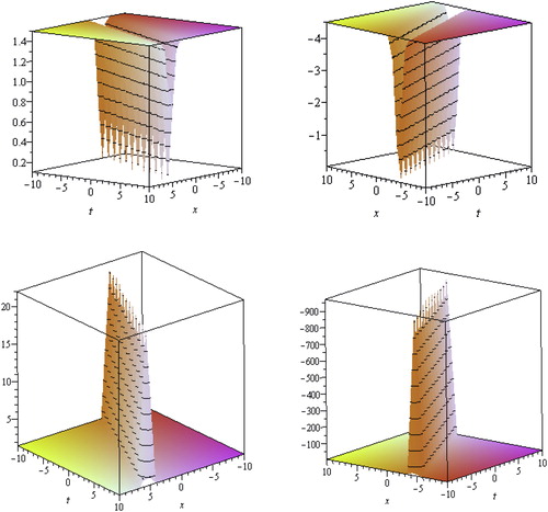
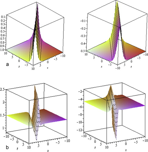
. Solitons have a remarkable property-- it keeps its identity upon interacting with other solitons. Soliton solutions also give rise to particle-like structures, such as magnetic monopoles etc. Fig. 1 presented the soliton obtained from solutions
,
and
withp=−c/2, q=1, λ=1, μ=−1, d=1.5, ν=3, α−1=2 and −10≤x, t≤10, y=0 respectively.
Solutions of ,
and
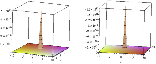
represents the single soliton solution. In Fig. 2, we have presented the single soliton solutions of
and
forp=−c/2, q=1, λ=1, μ=−1, ν=3, α−1=2 with −10≤x, t≤10, y=0 respectively.
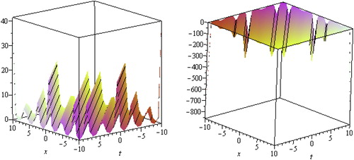
Solutions,
,
,
,
,
,
and
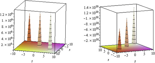
describes the multiple soliton solutions. In Fig. 3, we have presented the multiple soliton solutions of
,
forp=−c/2, q=1, λ=1, μ=−1, ν=3, α1=1 with −10≤x, t≤10, y=0 respectively.
Solutions of ,
,
and
are Cuspon of the Maccari system Equation(8)
(8)
(8) . Cuspons are other forms of solitons where solution exhibits cusps at their crests. Unlike peakons where the derivatives at the peak differ only by a sign, the derivatives at the jump of a cuspon diverge. The statement is that cuspon can be represented as
. It can easily be shown that
at the cusp, and
,
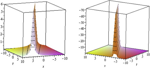
to distinguish the soliton property. In Fig. 4, we presented the shape of the cuspon, obtain from solutions
and
of the Maccari system Equation(8)
(8)
(8) forλ=0, μ=0, ν=3, d=1, α−1=2, c1=0.5 with −10≤x, t≤10,y=0 respectively.
Solutions ,
,
and
are bell-shape
solitary traveling wave solution. The Fig. 5 shows the shape of bell-shaped
solitary traveling wave solution (only shows the shape of solution of
and
only for p=−c/2, p=1, k=5, λ=1, μ=0, ν=3, d=1, α−1=2 with −10≤x, t≤10, y=0.
Singular kink solution is another kind of travelling wave solution which comes from infinity as in trigonometry. The solution of
and
comes infinity as in trigonometry, are singular kink solution. The Fig. 5 shows the shape of the exact singular kink-type solution (only shows the shape of solution of
forp=−c/2, q=1, λ=1, μ=−1, ν=3, d=1.5, α−1=2 with −10≤x, t≤10,y=0 ).
Solutions of and
represent the exact periodic traveling wave solutions. Periodic solutions are traveling wave solutions that are periodic such as cos(x−t). In Fig. 6, we have represented the periodic solution of
and
for p=−c/2, q=1, λ=−1, μ=1, ν=2, d=1, α1=1 with −10≤x, t≤10.
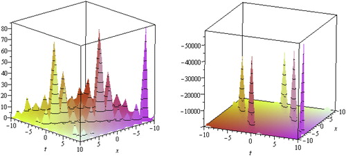
Solutions of to
are represented the exact soliton periodic traveling wave solutions of the Maccari system Equation(8)
(8)
(8) . In Fig. 7, we have presented soliton periodic traveling wave solution of
for p=−c/2, q=1, λ=−1, μ=1, ν=3, d=1, α−1=2 with −10≤x, t≤10, y=0 respectively.
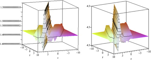
Solutions of
and
are represented the exact singular kink periodic traveling wave solutions of the Maccari system Equation(8)
(8)
(8) . In Fig. 8, we have presented singular kink periodic traveling wave solution of
and
for p=−c/2, q=1, λ=1, μ=−1, ν=3, d=1.5, α−1=2 with −10≤x, t≤10,y=0 respectively.
5 Conclusion
In this article, we have investigated a system of complex coupled equation. The novel (G′/G)-expansion method has been successfully applied to find more general travelling wave solutions of the coupled complex system. From the above solutions, we observe that if we take the particular values for the physical parameters, then these solutions are identical with the some particular solutions obtained by other methods and give us more new exact solutions than the other existing methods. A variety of distinct physical structures such as soliton solution, singular soliton solution, cuspon, kink type solution, singular kink solution, periodic solution, bell type solitary wave solution and solitary wave solutions are formally derived. The various types of exact travelling wave solutions provide the mathematical foundation in physics and engineering. Therefore, it is examined that the novel (G′/G)-expansion method would be a vital mathematical tool for solving not only a single NLEEs but also the coupled NLEEs.
Notes
Peer review under responsibility of Mansoura University.
References
- S.J.RussellReport on waves, in proceedings of the 14th meeting of the British Association for the advancement of science1844
- M.J.AblowitzP.A.ClarksonSoliton, nonlinear evolution equations and inverse scattering1991Cambridge University Press
- R.HirotaThe direct method in soliton theory2004Cambridge University Press
- V.B.MatveevM.A.SalleDarboux transformation and solitons1991SpringerBerlin
- R.HirotaR.BulloughP.CaudreyDirect method of finding exact solutions of nonlinear evolution equations, Backlund transformations1980SpringerBerlin11571175
- W.MalflietW.HeremanThe tanh method: II. Perturbation technique for conservative systemsPhys Scr541996569575
- W.MalflietW.HeremanThe tanh method: I. Exact solutions of nonlinear evolution and wave equationsPhys Scr541996563568
- G.W.BlumanS.KumeiSymmetries and differential equations1989Springer-VerlagBerlin
- J.WeissM.TaborG.CarnevaleThe Painlevé property for partial differential equationsJ Math Phys241983522
- M.A.AkbarN.H.M.AliNew solitary and periodic solutions of nonlinear evolution equation by exp-function methodWorld Appl Sci J1712201216031610
- H.NaherA.F.AbdullahM.A.AkbarNew traveling wave solutions of the higher dimensional nonlinear partial differential equation by the Exp-function methodJ Appl Math20121410.1155/2012/575387 article ID 575387
- T.ÖzişC.KöroğluA novel approach for solving the Fisher equation using Exp-function methodPhys Lett A37221200838363840
- C.KöroğluT.ÖzişA novel traveling wave solution for Ostrovsky equation using Exp-function methodComput Math Appl58200921422146
- T.ÖzişC.KöroğluA novel approach for solving the Fisher equation using Exp-function method Reply to: “Comment on:Phys Lett A373200911981200
- A.M.WazwazPartial differential equations: method and applications2002Taylor and Francis
- M.WangSolitary wave solutions for variant Boussinesq equationsPhy Lett A1991995169172
- W.WangX.LiJ.ZhangThe (G′/G)-expansion method and traveling wave solutions of nonlinear evolution equations in mathematical physicsPhys Lett A3722008417423
- J.ZhangX.WeiY.LuA generalized (G′/G)-expansion method and its applicationsPhys Lett A372200836533658
- J.ZhangF.JiangX.ZhaoAn improved (G′/G)-expansion method for solving nonlinear evolution equationsInt J Com Math878201017161725
- E.M.E.ZayedNew traveling wave solutions for higher dimensional nonlinear evolution equations using a generalized (G′/G)-expansion methodJ Phys A: Math Theor422009195202195214
- E.M.E.ZayedThe (G′/G)-expansion method combined with the Riccati equation for finding exact solutions of nonlinear PDEsJ Appl Math Informatics291–22011351367
- M.A.AkbarN.H.M.AliE.M.E.ZayedA generalized and improved (G′/G)-expansion method for nonlinear evolution equationsMath Prob Engr1220122210.1155/2012/459879
- M.N.AlamM.A.AkbarS.T.Mohyud-DinA novel (G′/G)-expansion method and its application to the Boussinesq equationChin Phys B2322014020203
- J.LeeR.SakthivelExact travelling wave solutions for some important nonlinear physical modelsPramana – J Phys802013757769
- M.G.HafezM.N.AlamM.A.AkbarTraveling wave solutions for some important coupled nonlinear physical models via the coupled Higgs equation and the Maccari systemJ King Saud Uni Sci272015105112
- J.ManafianI.ZamanpourAnalytical treatment of the coupled Higgs equation and Maccari system via Exp-function methodActa Univ Apulensis332013203216
- J.ManafianI.ZamanpourModification of truncated expansion method to some complex nonlinear partial differential equationsActa Univ Apulensis332013109216
- S.ZhuThe generalized Riccati equation mapping method in non-linear evolution equation: application to (2+1)-dimensional Boiti-Leon-Pempinelle equationChaos Solit Fract37200813351342
- M.A.AkbarN.H.M.AliS.T.Mohyud-DinThe alternative (G′/G)-expansion method with generalized Riccati equation: application to fifth order (1+1)-dimensional Caudrey-Dodd-Gibbon equationInt J Phys Sci752012743752
- E.M.E.ZayedThe (G′/G)-expansion method and its applications to some nonlinear evolution equations in the mathematical physicsJ Appl Math Comput30200989103