Time-fractional effect on pressure waves propagating through a fluid filled circular long elastic tube

Dedicated to Prof. S. A. El-Wakil for his Diamond Birthday.

PACS: 47.53. + n; 05.30.Pr; 83.50.-v.

Abstract

The pressure waves propagating through an incompressible inviscid fluid that moves in a circular cylindrical long elastic tube are considered. The reductive perturbation method is used to derive the KdV equation from the hydrodynamic equations of the system. The Euler–Lagrange variational technique described by Agrawal has been applied to formulate the time-fractional KdV equation. The derived time-fractional KdV equation is solved by employing the variational-iteration method represented by He. The effects of the tube and fluid parameters and the time fractional order on the propagation of pressure waves are investigated.

Keywords:

• Pressure waves
• Incompressible inviscid fluid
• Euler–Lagrange variational technique
• Time-fractional KdV equation
• Variational-iteration method

1 Introduction

The propagation of pressure waves in fluid that moves in large vessels was studied by many authors, e.g. References 1–^{[2][3][4][5][6][7][8][9][10][11][12][13][14][15]}16. Many of the works studied the small amplitude wave propagation in elastic tubes, ignored the nonlinear effects and focused on the dispersive characteristic [3–^[4]5]. When the nonlinear character appears, either finite amplitude or small-but-finite amplitude wave is considered, depending on the nonlinearity order. The propagation of finite waves through fluid filled elastic or viscoelastic tubes was studied [6–^[7]9]. Also, the small-but-finite amplitude waves propagating in distensible tubes were investigated [10–^[11]16], where the Korteweg–de Vries (KdV) equation appears due to the balancing between the nonlinearity and the dispersion effects.

The KdV equation as evolution and interaction model of nonlinear waves is employed to represent a wide range of physical phenomena. The KdV equation was first formulated as an evolution equation governing one-dimensional, small amplitude, long surface gravity waves propagating in a shallow water channel [17]. Afterward, the KdV equation has appeared in a number of other physical problems such as ion-acoustic waves, collision-free hydro-magnetic waves, plasma physics, stratified internal waves, lattice dynamics, etc. [18]. By means of the KdV model, some theoretical physics phenomena in quantum mechanics domain and continuum mechanics for shock wave formation are explained. The KdV model is also applied in many scientific fields like fluid dynamics, aerodynamics, solitons, turbulence, boundary layer behavior and mass transport.

Most of the forces in nature are non-conservative: dissipative and/or dispersive forces. The classical mechanics treated conservative forces using integer differential equations, while the non-conservative forces can be described in terms of the non-integer differential equations. Non-integer differentiation and integration is called Fractional Calculus, which is a field of mathematics study that generalizes the traditional definitions of calculus integral and derivative operators. During the last decades, Fractional Calculus has acquired importance due to its applications in various fields of science and engineering, including electrical networks, signal processing, optics, fluid flow, viscoelasticity, rheology, probability and statistics, dynamical process in self-similar and porous structures, diffusive transport, control theory of dynamical systems, electrochemistry of corrosion, and so on [19–^{[20][21][22][23][24][25][27][28][29][30][31][32][33][34][35]}35].

Riewe [19,20] used fractional derivatives [21–^[22]23] in the action to have non-conservative Euler–Lagrange equations. In terms of Riemann–Liouville fractional derivatives, Agrawal [24–^[25]26] used variational technique to formulate fractional equations of motion. These Euler–Lagrange equations are employed to investigate different real problems [27–^{[28][29][30][31][32][33][34][35]}35].

The fractional differential equations are solved by applying several methods such as: Fourier transformation method, Laplace transformation method, operational method, and the iteration method [21–^[22]23]. However, most of these methods are suitable only for special types of fractional differential equations, called linear with constant coefficients. Recently, there are some works dealing with the solutions of nonlinear fractional differential equations using techniques of nonlinear analysis such as: Adomian decomposition method (ADM) [36–^{[37][38][39][40][41]}42], variational-iteration method (VIM) [43–^[44]48], homotopy perturbation method (HPM) [49,50] and others. Adomian decomposition method [36–^[37]38] succeeded to solve accurately different types of fractional nonlinear differential equations by applying the Adomian polynomials. This method is applied to study many problems arising from applied sciences and engineering [39–^[40]42]. The variational-iteration method [43–^[44]46] was successfully employed to solve many types of linear, nonlinear and fractional differential equations that describe scientific and engineering problems [46–^[47]48]. As advantages over ADM, the VIM solves differential equations without using Adomian polynomials and has no linearization or perturbation for solving the nonlinear and fractional problems. The VIM principles for solving the differential equations are given in many papers, e.g. References 46–^[47]48. The VIM solution is provided as a convergent series, which may lead to exact solution for linear differential equations and to an efficient numerical solution for nonlinear and fractional differential equations. The series solution begins with a trial function that can be used as the solution of the linear term of the differential equation.

Our main motive here is to study the time fractional parameter effects on the propagation of solitary pressure waves through a fluid filled elastic tube. Therefore, beside what is considered in Reference 16, the derived nonlinear KdV equation is transformed using variational technique described by Agrawal [24–^[25]26] into the time fractional KdV (TFKdV) equation [45]. The TFKdV equation is solved by applying VIM [46–^[47]48] developed by He and the effect of the fractional order is studied.

This paper is organized as follows: The basic set of tube and fluid equations, which governs our system, is presented in section 2. In section 3, the KdV equation is derived by applying the reductive perturbation method [51]. Section 4 is devoted to derive and solve the time fractional KdV (TFKdV) equation using variational methods. Finally, some results and discussion are presented in section 5.

2 Basic equations of motion of the tube and fluid

A circular cylindrical long tube of un-deformed radius $R_0$, subjected to a uniform initial inner pressure $P_0$ is considered. A position vector $\underset{¯}{r}$ of a general point on the tube is described as [11,12]:(1a) $\underset{¯}{r}=[r_0+u(z,t)]{\underset{¯}{\widehat{e}}}_r+z{\underset{¯}{\widehat{e}}}_z$(1a) (1b) $z={\lambda }_{z}Z$(1b) where $r_0$ is the radius of the tube after a finite static deformation, $u(z,t)$ is a finite dynamic time dependent deformation in the tube radius, ${\underset{¯}{\widehat{e}}}_r$ and ${\underset{¯}{\widehat{e}}}_z$ are the radial and axial unit vectors, respectively in the cylindrical polar coordinates. $Z$ is the axial coordinate before the deformation, $z$ is the axial coordinate after the static deformation and ${\lambda }_z$ is the axial stretch ratio. The equation of motion of a small element of the tube's wall in the radial direction is given by [11,12](2) $\begin{array}{c}\frac{R_0{\rho }_0}{{\lambda }_z}\frac{{\partial }^{2}u(z,t)}{\partial t^2}=\frac{\partial }{\partial z}\left[\frac{R_0\mu }{\Lambda }\frac{\partial {\displaystyle \sum (z,t)}}{\partial {\lambda }_1}\frac{\partial u(z,t)}{\partial z}\right]\\ -\frac{\mu }{{\lambda }_z}\frac{\partial {\displaystyle \sum (z,t)}}{\partial {\lambda }_2}+\frac{R_0{\lambda }_2}{H}P*\left(z,t\right)\end{array}$(2) where ${\rho }_0$ and $\mu$ are the mass density and the shear modulus of the tube material, respectively. $\sum (z,t)$ is the strain energy density function, $P*(z,t)$ is the fluid pressure at the final inner deformed tube radius $r_f$ and $H$ is the initial un-deformed tube thickness. $r$ and $z$ are the radial and axial cylindrical coordinates, respectively after both static and dynamic deformations and $t$ is the time parameter. ${\lambda }_1$ and ${\lambda }_2$ are the axial and radial direction stretches, respectively and are represented by [11,12](3a) ${\lambda }_1={\lambda }_z\Lambda$(3a) (3b) ${\lambda }_2={\lambda }_r+u(z,t)/R_0$(3b) (3c) $\Lambda ={\{1+{[\partial u(z,t)/\partial z]}^2\}}^{1/2}$(3c) where ${\lambda }_r=r_0/R_0$ is the radial stretch ratio after finite static deformation.

Equation (2)(2) $\begin{array}{c}\frac{R_0{\rho }_0}{{\lambda }_z}\frac{{\partial }^{2}u(z,t)}{\partial t^2}=\frac{\partial }{\partial z}\left[\frac{R_0\mu }{\Lambda }\frac{\partial {\displaystyle \sum (z,t)}}{\partial {\lambda }_1}\frac{\partial u(z,t)}{\partial z}\right]\\ -\frac{\mu }{{\lambda }_z}\frac{\partial {\displaystyle \sum (z,t)}}{\partial {\lambda }_2}+\frac{R_0{\lambda }_2}{H}P*\left(z,t\right)\end{array}$(2) has been derived by applying Newton's second law of motion for a small element of the tube wall material [11,12]. The term in the left hand side is Newton's second law force of the wall element. In the right hand side, the first term is the force due to axial tension of the tube wall, the second term is the force due to the tension in the radial direction and the third term is the force due to the inner fluid pressure on the tube wall element.

The value of the fluid pressure at the final radius of the deformed tube ($r_f$) can be obtained from (2) as(4) $\begin{array}{c}P*(z,t)=\frac{{\rho }_{0}H}{{\lambda }_1{\lambda }_2}\frac{{\partial }^{2}u(z,t)}{\partial t^2}+\frac{\mu H}{{\lambda }_1{\lambda }_2{R}_0}\frac{\partial {\displaystyle \sum (z,t)}}{\partial {\lambda }_2}\\ -\frac{\mu H{\lambda }_z}{{\lambda }_1{\lambda }_2}\frac{\partial }{\partial z}\left[\frac{1}{\Lambda }\frac{\partial {\displaystyle \sum (z,t)}}{\partial {\lambda }_1}\frac{\partial u(z,t)}{\partial z}\right]\end{array}$(4)

On the other hand, the fluid that filled the tube is considered to be an incompressible inviscid fluid. The ratio of the viscous term to the nonlinear term is assumed to be very small. Therefore, the viscous effect in comparison to the nonlinear effect will be neglected. Based on these assumptions, the incompressible inviscid fluid filled the tube has equations of axially symmetrical motion in the cylindrical polar coordinates represented by [12,13](5a) $\frac{\partial V(r,z,t)}{\partial r}+\frac{V(r,z,t)}{r}+\frac{\partial W(r,z,t)}{\partial z}=0$(5a) (5b) $\begin{array}{l}\frac{\partial V(r,z,t)}{\partial t}+V(r,z,t)\frac{\partial V(r,z,t)}{\partial r}\\ +W(r,z,t)\frac{\partial V(r,z,t)}{\partial z}+\frac{1}{{\rho }_f}\frac{\partial P(r,z,t)}{\partial r}=0\end{array}$(5b) (5c) $\begin{array}{l}\frac{\partial W(r,z,t)}{\partial t}+V(r,z,t)\frac{\partial W(r,z,t)}{\partial r}\\ +W(r,z,t)\frac{\partial W(r,z,t)}{\partial z}+\frac{1}{{\rho }_f}\frac{\partial P(r,z,t)}{\partial z}=0\end{array}$(5c)

The first equation (5a)(5a) $\frac{\partial V(r,z,t)}{\partial r}+\frac{V(r,z,t)}{r}+\frac{\partial W(r,z,t)}{\partial z}=0$(5a) is the incompressibility condition (mass conservation) of the fluid, while (5b)(5b) $\begin{array}{l}\frac{\partial V(r,z,t)}{\partial t}+V(r,z,t)\frac{\partial V(r,z,t)}{\partial r}\\ +W(r,z,t)\frac{\partial V(r,z,t)}{\partial z}+\frac{1}{{\rho }_f}\frac{\partial P(r,z,t)}{\partial r}=0\end{array}$(5b) and (5c)(5c) $\begin{array}{l}\frac{\partial W(r,z,t)}{\partial t}+V(r,z,t)\frac{\partial W(r,z,t)}{\partial r}\\ +W(r,z,t)\frac{\partial W(r,z,t)}{\partial z}+\frac{1}{{\rho }_f}\frac{\partial P(r,z,t)}{\partial z}=0\end{array}$(5c) are conservative equations of fluid momentum in radial and axial directions, respectively.

These field equations (5) satisfy boundary conditions at the wall as follows:

The pressure at the final deformed radius of the tube is given as(6a) $P(r_f\text{},z,t)=P*(z,t)$(6a) while the fluid velocity at the wall is assumed to equal the radial velocity of the wall itself (no-slip condition) [13], so(6b) $V(r_f\text{},z,t)={\frac{d\underset{¯}{r}}{dt}\cdot {\underset{¯}{\widehat{e}}}_r|}_{r=r_f}=\frac{\partial u(z,t)}{\partial t}+\frac{\partial u(z,t)}{\partial z}W(r_f\text{},z,t)$(6b)

Here $V(r,z,t)$ and $W(r,z,t)$ are the radial and axial fluid velocity components, respectively, $P(r,z,t)$ is the fluid pressure and ${\rho }_f$ is the fluid mass density.

The strain energy density $\sum (z,t)$ is generally a function of ${\lambda }_1$ and ${\lambda }_2$. Expanding $\sum (z,t)$ into power series at its equilibrium, (4) can take the form [16](7) $\begin{array}{c}P*(z,t)=\frac{b_1\mu H}{R_0^2}u+\frac{{\rho }_{0}H}{{\lambda }_r{\lambda }_z}\frac{{\partial }^{2}u}{\partial t^2}-a_1\mu H\frac{{\partial }^{2}u}{\partial z^2}+\frac{b_2\mu H}{R_0^3}{u}^2-\frac{{\rho }_{0}H}{{\lambda }_r^2{\lambda }_z{R}_0}u\frac{{\partial }^{2}u}{\partial t^2}\\ -\frac{a_2\mu H}{R_0}{\left(\frac{\partial u}{\partial z}\right)}^2+\left(\frac{a_1\mu H}{{\lambda }_r{R}_0}-\frac{2a_2\mu H}{R_0}\right)u\frac{{\partial }^{2}u}{\partial z^2}+\frac{\mu H}{R_0}{P}_0\end{array}$(7) where the coefficients $a_1$, $a_2$, $b_1$ and $b_2$ are defined by(8a) $a_1={\frac{1}{{\lambda }_r{\lambda }_z}\frac{\partial \sum }{\partial \Lambda }|}_{u=0}\text{},a_2={\frac{R_0}{{\lambda }_r{\lambda }_z}\frac{{\partial }^2\sum }{\partial \Lambda \partial u}|}_{u=0}$(8a) (8b) $b_1={\frac{R_0}{{\lambda }_r{\lambda }_z}\left(R_0\frac{{\partial }^2\sum }{\partial u^2}-\frac{1}{{\lambda }_r}\frac{\partial \sum }{\partial u}\right)|}_{u=0}\text{},b_2={\frac{R_0^3}{2{\lambda }_r{\lambda }_z}\frac{{\partial }^3\sum }{\partial u^3}|}_{u=0}-\frac{b_1}{{\lambda }_r}$(8b)

Equations (5)–(7) give sufficient relations to determine the unknowns $V(r,z,t)$, $W(r,z,t)$, $u(r,z,t)$, and $P(r,z,t)$.

3 The Evolution equation

The following stretched co-ordinates can be introduced by applying the reductive perturbation theory [51] as:(10) $\xi ={\epsilon }^{1/2}(z-gt),\tau ={\epsilon }^{3/2}t$(10) where $\epsilon$ is a smallness parameter and $g$ is the long wave approximation's phase velocity. The physical quantities represented in (5)–(8) are expanded as power series in $\epsilon$ as:(11a) $V(r,\xi ,\tau )={\epsilon }^{3/2}{V}_1(r,\xi ,\tau )+{\epsilon }^{5/2}{V}_2(r,\xi ,\tau )+{\epsilon }^{7/2}{V}_3(r,\xi ,\tau )+\dots$(11a) (11b) $W(r,\xi ,\tau )=\epsilon W_1(r,\xi ,\tau )+{\epsilon }^2{W}_2(r,\xi ,\tau )+{\epsilon }^3{W}_3(r,\xi ,\tau )+\dots$(11b) (11c) $P(r,\xi ,\tau )=\epsilon P_1(r,\xi ,\tau )+{\epsilon }^2{P}_2(r,\xi ,\tau )+{\epsilon }^3{P}_3(r,\xi ,\tau )+\dots$(11c) (11d) $u(\xi ,\tau )=\epsilon u_1(\xi ,\tau )+{\epsilon }^2{u}_2(\xi ,\tau )+{\epsilon }^3{u}_3(\xi ,\tau )+\dots$(11d)

Substituting (10) and (11) into (5) and (6), applying (7) and equating the coefficients of different powers of $\epsilon$, the following results are obtained:

The coefficient of the first-order of $\epsilon$ is(12a) $\frac{1}{{\rho }_f}\frac{\partial P_1(r,\xi ,\tau )}{\partial r}=0$(12a) with the boundary condition(12b) ${P_1(r,\xi ,\tau )|}_{r=r_f}=(b_1\mu H/R_0^2)u_1(\xi ,\tau )$(12b)

Meanwhile, the coefficients of ${\epsilon }^{3/2}$ are given as(13a) $\frac{1}{{\rho }_f}\frac{\partial P_1(r,\xi ,\tau )}{\partial \xi }-g\frac{\partial W_1(r,\xi ,\tau )}{\partial \xi }=0$(13a) (13b) $\frac{\partial V_1(r,\xi ,\tau )}{\partial r}+\frac{V_1(r,\xi ,\tau )}{r}+\frac{\partial W_1(r,\xi ,\tau )}{\partial \xi }=0$(13b) with boundary condition(13c) ${V_1(r,\xi ,\tau )|}_{r=r_f}=-g[\partial u_1(\xi ,\tau )/\partial \xi ]$(13c) where(13d) $g^2=b_1\mu H{r}_f/(2{\rho }_0{R}_0^2)$(13d)

The coefficient of ${\epsilon }^2$ gives the following equation(14a) $\frac{\partial P_2}{\partial r}-g{\rho }_f\frac{\partial V_1}{\partial \xi }=0$(14a) under the boundary condition(14b) ${P_2|}_{r=r_f}=\left(\frac{{\rho }_{0}H{g}^2}{{\lambda }_r{\lambda }_z}-a_1\mu H\right)\frac{{\partial }^2{u}_1}{\partial {\xi }^2}+\frac{b_2\mu H}{R_0^3}{u}_1^2+\frac{b_1\mu H}{R_0^2}{u}_2$(14b)

The coefficients of ${\epsilon }^{5/2}$ are given in the forms(15a) $\frac{\partial V_2}{\partial r}+\frac{V_2}{r}+\frac{\partial W_2}{\partial \xi }=0$(15a) (15b) $\frac{\partial W_1}{\partial \tau }+V_1\frac{\partial W_1}{\partial r}+W_1\frac{\partial W_1}{\partial \xi }+\frac{1}{{\rho }_f}\frac{\partial P_2}{\partial \xi }-g\frac{\partial W_2}{\partial \xi }=0$(15b)

with the boundary condition(15c) ${V_2|}_{r=r_f}=\frac{\partial u_1}{\partial \tau }+W_1\frac{\partial u_1}{\partial \xi }-g\frac{\partial u_2}{\partial \xi }$(15c)

Eliminating the second order perturbation quantities $P_2$, $V_2$, $W_2$ and $u_2$ in (14) and (15) employing (12) and (13) to define the first order perturbation quantities $V_1$, $W_1$ and $u_1$ lead to KdV equation for the first-order perturbation pressure $P_1$ in the form:(16) $\frac{\partial }{\partial \tau }Y(\xi ,\tau )+AY(\xi ,\tau )\frac{\partial }{\partial \xi }Y(\xi ,\tau )+B\frac{{\partial }^3}{\partial {\xi }^3}Y(\xi ,\tau )=0$(16) where $Y(\xi ,\tau )$ represents the first-order perturbation pressure $P_1$. The nonlinear coefficient $A$ and dispersion coefficient $B$ are defined, respectively by(17a) $A=g{R}_0(2R_0{b}_1+b_2{r}_f)/(b_1^2\mu H{r}_f)$(17a) (17b) $B=(g/2)[{\rho }_{0}H{r}_f/(2{\rho }_f{\lambda }_r{\lambda }_z)-a_1{R}_0^2/b_1+r_f^2/8]$(17b)

To study the effect of time fractional derivative on the pressure pulses propagation in inviscid non-Newtonian incompressible fluid, the KdV equation (16)(16) $\frac{\partial }{\partial \tau }Y(\xi ,\tau )+AY(\xi ,\tau )\frac{\partial }{\partial \xi }Y(\xi ,\tau )+B\frac{{\partial }^3}{\partial {\xi }^3}Y(\xi ,\tau )=0$(16) must be represented in terms of time-fractional form as in the following section.

4 Time-fractional KdV equation and its solution

The TFKdV equation in (1 + 1) dimension can be formulated following El-Wakil et al. [45] to have the form [see Appendix A]:(18) $\begin{array}{l}{}_0{}^R\text{}{D}_{\tau }^{\alpha }Y(\xi ,\tau )+AY(\xi ,\tau )\frac{\partial }{\partial \xi }Y(\xi ,\tau )+B\frac{{\partial }^3}{\partial {\xi }^3}Y(\xi ,\tau )=0,\\ 0<\alpha \le 1,\tau \in [0,T_0]\end{array}$(18)

where the Riesz fractional operator ${}_0{}^R\text{}{D}_{\tau }^{\alpha }U(\xi ,\tau )$ is represented by [21–^[22]23](19) $\begin{array}{c}{}_0{}^R\text{}{D}_{\tau }^{\alpha }f(\xi ,\tau )=\frac{1}{2}\frac{1}{\Gamma (1-\alpha )}\frac{d}{d\tau }\left[{\displaystyle {\int }_0^{\tau }dt{(\tau -t)}^{-\alpha }f(\xi ,t)}-{\displaystyle {\int }_{\tau }^{T_0}dt{(t-\tau )}^{-\alpha }f(\xi ,t)}\right]\\ =\frac{1}{2}\frac{1}{\Gamma (1-\alpha )}\frac{d}{d\tau }{\displaystyle {\int }_0^{T_0}dt{\left|\tau -t\right|}^{-\alpha }f(\xi ,t)}\end{array}$(19)

The TFKdV equation represented by (18) can be solved using the VIM [43–^[44][45]46] in terms of the following correction functional [see Appendix B](20) $\begin{array}{c}{Y}_{n+1}(\xi ,\tau )=Y_n(\xi ,\tau )\\ -{\displaystyle {\int }_0^{\tau }d{\tau }^{\prime }\{\frac{\partial }{\partial {\tau }^{\prime }}{Y}_n(\xi ,{\tau }^{\prime })-{{}_0^R\text{}{I}_{{\tau }^{\prime }}^{1-\alpha }{Y}_n(\xi ,{\tau }^{\prime })|}_{{\tau }^{\prime }=0}[{{\tau }^{\prime }}^{(\alpha -2)}/\Gamma (\alpha -1)]}\\ +{}_0^R{D}_{{\tau }^{\prime }}^{1-\alpha }\left[A{Y}_n(\xi ,\tau )\frac{\partial }{\partial \xi }{Y}_n(\xi ,{\tau }^{\prime })+B\frac{{\partial }^3}{\partial {\xi }^3}{Y}_n(\xi ,{\tau }^{\prime })\right]\},n\ge 0\end{array}$(20)

where the Riesz integral operator ${}_a{}^R\text{}{I}_{\tau }^{\alpha }Y(\xi ,\tau )$ is represented by [21–^[22]23](21) ${}_a{}^R\text{}{I}_{\tau }^{\alpha }f(\xi ,\tau )=\frac{1}{2}\frac{1}{\Gamma (\alpha )}{\displaystyle {\int }_a^{b}dt{\left|\tau -t\right|}^{\alpha -1}f(\xi ,t)}$(21)

If the parameter $\tau$ represents the time-variable in (18), the right Riemann–Liouville fractional derivative in Riesz fractional operator can be interpreted as future states of the system. Therefore, this term may be neglected in calculations, when the present state of the system does not depend on the results of the future development [23].

The initial value of the state variable can be taken to represent the zero-order correction of the solution. This initial value is taken as the solution of the ordinary KdV equation at time equal to zero, in this case as:(22a) $Y_0(\xi ,\tau )=Y(\xi ,0)=A_0\sec {\mathrm{h}}^2(c\xi )$(22a) where $A_0=3v/A$, $c=\sqrt{v/(4B)}$.

Substituting the zero-order solution (22a) into (20) leads to the first order approximation as(22b) $\begin{array}{c}{Y}_1(\xi ,\tau )=A_0\sec {\mathrm{h}}^2(c\xi )+2A_{0}c\sinh (c\xi )\sec {\mathrm{h}}^3(c\xi )\\ \ast [4c^{2}B+(A_{0}A-12c^{2}B)\sec h^2(c\xi )]{\tau }^{\alpha }/\Gamma (\alpha +1)\end{array}$(22b)

Substituting this equation into (20) and using the Mathematical package like Maple or Mathematica lead to the second order approximation in the form(22c) $\begin{array}{c}{Y}_2(\xi ,\tau )=A_0\sec {\mathrm{h}}^2(c\xi )+2A_{0}c\sinh (c\xi )\sec \mathrm{h}{(c\xi )}^3\\ \ast [4c^{2}B+(A_{0}A-12c^{2}B)\sec \mathrm{h}{(c\xi )}^2]\frac{{\tau }^{\alpha }}{\Gamma (\alpha +1)}\\ +2A_0{c}^2\sec \mathrm{h}{(c\xi )}^2[32c^4{B}^2\\ +16c^{2}B(5A_{0}A-63c^{2}B)\sec \mathrm{h}{(c\xi )}^2\\ +2(3A_0^2{A}^2-176A_0{c}^{2}AB+1680c^4{B}^2)\sec \mathrm{h}{(c\xi )}^4\\ -7(A_0^2{A}^2-42A_0{c}^{2}AB+360c^4{B}^2)\sec \mathrm{h}{(c\xi )}^6]\frac{{\tau }^{2\alpha }}{\Gamma (2\alpha +1)}\\ +4A_0^2{c}^3\sinh (c\xi )\sec \mathrm{h}{(c\xi )}^5[32c^4{B}^2\\ +24c^{2}B(A_{0}A-14c^{2}B)\sec \mathrm{h}{(c\xi )}^2\\ +4(A_0^2{A}^2-32A_0{c}^{2}AB+240c^4{B}^2)\sec \mathrm{h}{(c\xi )}^4\\ -5(A_0^2{A}^2-24A_0{c}^{2}AB+144c^4{B}^2)\sec \mathrm{h}{(c\xi )}^6]\\ \frac{\Gamma (2\alpha +1)}{{[\Gamma (\alpha +1)]}^2}\frac{{\tau }^{3\alpha }}{\Gamma (3\alpha +1)}\end{array}$(22c)

The higher order approximations can be calculated using a symbolic mathematical package to the appropriate order where the infinite approximation leads to exact solution.

5 Results and discussion

Blood is known to be an incompressible non-Newtonian fluid. The order of hematocrit ratio (red cell concentration) and the deformability of red blood cells are the main factors that make blood behave like a Newtonian fluid. Experimental observations show that blood behaves as a Newtonian fluid when the shear rate is high. Blood viscosity can be considered very small to be neglected with respect to its nonlinear term. Due to these observations, it can be assumed that blood can be treated as incompressible inviscid fluid.

The reductive perturbation method [51] is applied to drive the KdV equation for a system of fluid filled elastic tube. A variational method suggested by Agrawal [24–^[25]26] is used to derive the TFKdV equation. The VIM [43–^{[44][45][46][47]}48] developed by He [46] is employed to solve the derived equation by applying the Riemann–Liouville definition for the fractional derivative.

The numerical results are made physically relevant by applying parameters close to experimental data in dogs [52,53]. The average values of the parameters are founded experimentally as $R_0=0.38cm$, $H=0.02cm$, $\mu =0.4$, $r_f=0.75cm$, ${\rho }_0=1.03gm/c{m}^3$, ${\rho }_f=1.05gm/c{m}^3$, $a_1=78.692$, $b_1=296.105$, $b_2=991.496$, ${\lambda }_z={\lambda }_r=1.6$ and $v=8cm/s$. These experimental data are employed to study the pressure waves in dogs' blood and the wave forms are represented in different figures.

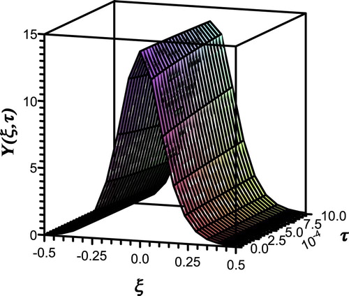
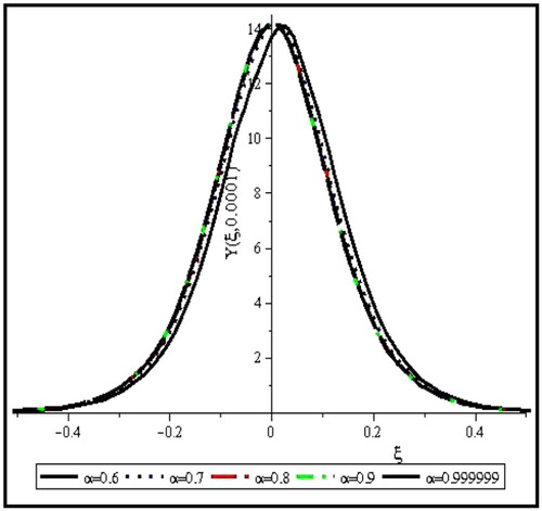
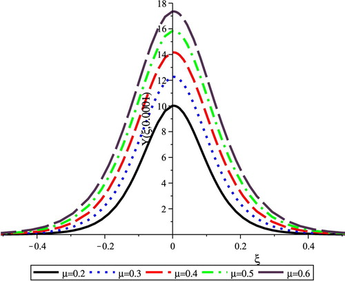
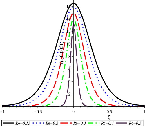
The pressure wave against space and time at fractional parameter $\alpha =0.8$ has soliton shape as presented in Fig. 1, which means that the pressure wave has constant shape through the artery. Effect of the variation of $\alpha$ on the pressure wave is studied in Fig. 2. This figure shows that the fractional order of differentiation has a small effect only on the position of the wave peak. The initial radius of the blood-vessel $R_0$ effect on the blood pressure wave is represented in Fig. 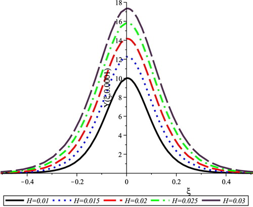3, which shows that the increase of $R_0$ decreases both the amplitude and width of the pressure wave. In Fig. 4, the increase of the thickness of the blood-vessel wall $H$ increases both of the amplitude and width of the blood pressure wave. The shear modulus of the blood-vessel wall material $\mu$ effect on the blood pressure waves is given in Fig. 5. 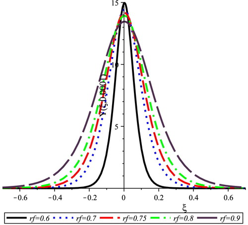It is shown that the increase of $\mu$ increases both the amplitude and width of the pressure wave. Figure 6 represents the effect of the final radius of the blood-vessel $r_f$ on the pressure waves. The representation shows that the increase of $r_f$ decreases the amplitude while it increases the width of the pressure wave.

Fig. 1 The pressure wave with position and time for $R_0=0.38cm$, $H=0.02cm$, $\mu =0.4$, $r_f=0.75cm$, ${\rho }_0=1.03gm/c{m}^3$, ${\rho }_f=1.05gm/c{m}^3$, $a_1=78.692$, $b_1=296.105$, $b_2=991.496$, ${\lambda }_z={\lambda }_r=1.6$, $v=8cm/s$ and $\alpha =0.8$.

Fig. 2 The pressure wave with position at different values of $\alpha$ for $R_0=0.38cm$, $H=0.02cm$, $\mu =0.4$, $r_f=0.75cm$, ${\rho }_0=1.03gm/c{m}^3$, ${\rho }_f=1.05gm/c{m}^3$, $a_1=78.692$, $b_1=296.105$, $b_2=991.496$, ${\lambda }_z={\lambda }_r=1.6$ and $v=8cm/s$.

Fig. 3 The pressure wave with position at different values of $R_0$ for $H=0.02cm$, $\mu =0.4$, $r_f=0.75cm$, ${\rho }_0=1.03gm/c{m}^3$, ${\rho }_f=1.05gm/c{m}^3$, $a_1=78.692$, $b_1=296.105$, $b_2=991.496$, ${\lambda }_z={\lambda }_r=1.6$, $v=8cm/s$ and $\alpha =0.8$.

Fig. 4 The pressure wave with position at different values of $H$ for $R_0=0.38cm$, $\mu =0.4$, $r_f=0.75cm$, ${\rho }_0=1.03gm/c{m}^3$, ${\rho }_f=1.05gm/c{m}^3$, $a_1=78.692$, $b_1=296.105$, $b_2=991.496$, ${\lambda }_z={\lambda }_r=1.6$, $v=8cm/s$ and $\alpha =0.8$.

Fig. 5 The pressure wave with position at different values of $\mu$ for $R_0=0.38cm$, $H=0.02cm$, $r_f=0.75cm$, ${\rho }_0=1.03gm/c{m}^3$, ${\rho }_f=1.05gm/c{m}^3$, $a_1=78.692$, $b_1=296.105$, $b_2=991.496$, ${\lambda }_z={\lambda }_r=1.6$, $v=8cm/s$ and $\alpha =0.8$.

Fig. 6 The pressure wave with position at different values of $r_f$ for $R_0=0.38cm$, $H=0.02cm$, $\mu =0.4$, ${\rho }_0=1.03gm/c{m}^3$, ${\rho }_f=1.05gm/c{m}^3$, $a_1=78.692$, $b_1=296.105$, $b_2=991.496$, ${\lambda }_z={\lambda }_r=1.6$, $v=8cm/s$ and $\alpha =0.8$.

The above calculations show that the blood-vessel characteristics modulate the shape of the pressure waves in the blood for both the amplitude and width while the fractional order of the evolution equation that describes the pressure wave propagation has a small effect on these waves.

Acknowledgements

All of the authors would like to pass their great thanks to their Professor S. A. El-Wakil, who is celebrating his Diamond Birthday, for his continuous encouragement, suggestions, and review of the work.

Notes

Dedicated to Prof. S. A. El-Wakil for his Diamond Birthday.

PACS: 47.53. + n; 05.30.Pr; 83.50.-v.

Appendix A

Time-fractional KdV-equation formulation

The TFKdV equation in (1 + 1) dimension can be formulated as follows [45]:

Using a potential function $V(\xi ,\tau )$ where $Y(\xi ,\tau )=V_{\xi }(\xi ,\tau )$ gives the potential equation of the regular KdV equation (16)(16) $\frac{\partial }{\partial \tau }Y(\xi ,\tau )+AY(\xi ,\tau )\frac{\partial }{\partial \xi }Y(\xi ,\tau )+B\frac{{\partial }^3}{\partial {\xi }^3}Y(\xi ,\tau )=0$(16) in the form(A1) $V_{\xi \tau }(\xi ,\tau )+A{V}_{\xi }(\xi ,\tau )V_{\xi \xi }(\xi ,\tau )+B{V}_{\mathit{\xi \xi \xi \xi }}(\xi ,\tau )=0$(A1)

The functional of this equation can be represented by(A2) $\begin{array}{c}J(V)={\displaystyle {\int }_{R}d\xi }{\displaystyle {\int }_{T}d\tau V(\xi ,\tau )[c_1{V}_{\xi \tau }(\xi ,\tau )}\\ +c_{2}A{V}_{\xi }(\xi ,\tau )V_{\xi \xi }(\xi ,\tau )+c_{3}B{V}_{\mathit{\xi \xi \xi \xi }}(\xi ,\tau )]\end{array}$(A2) where $c_1$, $c_2$, and $c_3$ are unknown constants to be determined. Integrating this equation by parts where ${V_{\xi }|}_R={V_{\tau }|}_T=0$ gives(A3) $\begin{array}{c}J(V)={\displaystyle {\int }_{R}d\xi }{\displaystyle {\int }_{T}d\tau \{[-c_1{V}_{\tau }(\xi ,\tau )V_{\xi }(\xi ,\tau )}\\ -\frac{1}{2}{c}_{2}A{[V_{\xi }(\xi ,\tau )]}^3+c_{3}B{[V_{\xi \xi }(\xi ,\tau )]}^2]\}\end{array}$(A3)

Taking the variation for the result with respect to $V(\xi ,\tau )$ leads to $c_1=\frac{1}{2}$, $c_2=\frac{1}{3}$, $c_3=\frac{1}{2}$.

So, the functional gives the Lagrangian of the potential equation as(A4) $L(V,V_{\tau }\text{},V_{\xi })=-\frac{1}{2}{V}_{\tau }(\xi ,\tau )V_{\xi }(\xi ,\tau )-\frac{1}{6}{c}_{2}A{[V_{\xi }(\xi ,\tau )]}^3+\frac{1}{2}B{[V_{\xi \xi }(\xi ,\tau )]}^2$(A4)

Similar to this form, the Lagrangian of the potential equation in the time-fractional domain can be written as(A5) $\begin{array}{c}F({}_0{D}_{\tau }^{\alpha }V,V,V_{\xi })=-\frac{1}{2}[{}_0{D}_{\tau }^{\alpha }V(\xi ,\tau )]V_{\xi }(\xi ,\tau )\\ -\frac{1}{6}A{[V_{\xi }(\xi ,\tau )]}^3+\frac{1}{2}B{[V_{\xi \xi }(\xi ,\tau )]}^2\end{array}$(A5)

where the left Riemann–Liouville fractional derivative ${}_0\text{}{D}_t^{\alpha }f(x,t)$ is represented by [21–^[22]23](A6) $\begin{array}{c}{}_a\text{}{D}_t^{\alpha }f(x,t)=\frac{1}{\Gamma (n-\alpha )}\frac{d^n}{d{t}^n}\left[{\displaystyle {\int }_a^{t}d\tau {(\tau -t)}^{n-\alpha -1}f(x,\tau )}\right],\\ t\in [a,b],n-1\le \alpha \le n\end{array}$(A6)

The functional of the time-fractional potential equation can be represented in the form(A7) $J(V)={\displaystyle {\int }_{R}dx}{\displaystyle {\int }_{T}dtF({}_0{D}_{\tau }^{\alpha }V,V,V_{\xi }\text{},V_{\xi \xi })}$(A7) where the time-fractional Lagrangian $F({}_0\text{}{D}_{\tau }^{\alpha }V,V,V_{\xi }\text{},V_{\xi \xi })$ is defined by (A5).

The variation of the functional with respect to $V(\xi ,\tau )$ leads to(A8) $\begin{array}{c}\delta J(V)={\displaystyle {\int }_{R}d\xi }{\displaystyle {\int }_{T}d\tau [\left(\frac{\partial F}{{\partial }_0{D}_{\tau }^{\alpha }V}\right){\delta }_0{D}_{\tau }^{\alpha }V+\left(\frac{\partial F}{\partial V_{\xi }}\right)\delta V_{\xi }}\\ +\left(\frac{\partial F}{\partial V}\right)\delta V+\left(\frac{\partial F}{\partial V_{\xi \xi }}\right)\delta V_{\xi \xi }]\end{array}$(A8)

Integrating the right-hand side of this equation by parts leads to(A9) $\delta J(V)={\displaystyle {\int }_{R}d\xi }{\displaystyle {\int }_{T}d\tau \left[{}_{\tau }{D}_{T_0}^{\alpha }\left(\frac{\partial F}{{\partial }_0{D}_{\tau }^{\alpha }V}\right)-\frac{\partial }{\partial \xi }\left(\frac{\partial F}{\partial V_{\xi }}\right)+\left(\frac{\partial F}{\partial V}\right)+\frac{{\partial }^2}{\partial {\xi }^2}\left(\frac{\partial F}{\partial V_{\xi }}\right)\right]\delta V}$(A9)

This is done by taking the fractional integrating by parts formula [21–^[22]23](A10) ${\displaystyle {\int }_a^{b}dtf{(t)}_a{D}_t^{\alpha }g(t)}={\displaystyle {\int }_a^{b}dtg{(t)}_t{D}_b^{\alpha }f(t)}$(A10) where the right Riemann–Liouville fractional derivative ${}_t\text{}{D}_b^{\alpha }f(x,t)$ is defined by [21–^[22]23](A11) $\begin{array}{c}{}_t\text{}{D}_b^{\alpha }f(x,t)=\frac{{(-1)}^n}{\Gamma (n-\alpha )}\frac{d^n}{d{t}^n}\left[{\displaystyle {\int }_t^{b}d\tau {(t-\tau )}^{n-\alpha -1}f(x,\tau )}\right],\\ t\in [a,b],n-1\le \alpha \le n\end{array}$(A11)

Optimizing this variation of the functional $J(V)$, i.e., $\delta J(V)=0$, gives the Euler–Lagrange equation for the time-fractional of the potential equation in the form(A12) ${}_{\tau }\text{}{D}_{T_0}^{\alpha }\left(\frac{\partial F}{{\partial }_0{D}_{\tau }^{\alpha }V}\right)-\frac{\partial }{\partial \xi }\left(\frac{\partial F}{\partial V_{\xi }}\right)+\left(\frac{\partial F}{\partial V}\right)+\frac{{\partial }^2}{\partial {\xi }^2}\left(\frac{\partial F}{\partial V_{\xi }}\right)=0$(A12)

Substituting from the Lagrangian equation into this Euler–Lagrange formula gives(A13) $-\frac{1}{2}[{}_{\tau }{D}_{T_0}^{\alpha }{V}_{\xi }(\xi ,\tau )]+\frac{1}{2}[{}_0{D}_{\tau }^{\alpha }{V}_{\xi }(\xi ,\tau )]+A{V}_{\xi }(\xi ,\tau )V_{\xi \xi }(\xi ,\tau )+B{V}_{\mathit{\xi \xi \xi \xi }}(\xi ,\tau )=0$(A13)

Substituting for the potential function $V_{\xi }(\xi ,\tau )=Y(\xi ,\tau )$ gives the time-fractional KdV equation for the state function $Y(\xi ,\tau )$ in the form(A14) $-\frac{1}{2}[{}_{\tau }{D}_{T_0}^{\alpha }Y(\xi ,\tau )]+\frac{1}{2}[{}_0{D}_{\tau }^{\alpha }Y(\xi ,\tau )]+AY(\xi ,\tau )Y_{\xi }(\xi ,\tau )+B{Y}_{\xi \xi \xi }(\xi ,\tau )=0$(A14) where the fractional derivatives ${}_0\text{}{D}_{\tau }^{\alpha }Y(\xi ,\tau )$ and ${}_{\tau }\text{}{D}_{T_0}^{\alpha }Y(\xi ,\tau )$ are the left and right Riemann–Liouville fractional derivatives respectively.

Appendix B

Time-fractional KdV equation solution

The TFKdV equation represented by (18) can be solved using the VIM [43–^{[44][45][46][47]}48] as follows:

Affecting from left by the fractional operator ${}_0^R\text{}{D}_{\tau }^{1-\alpha }$ on (18) leads to(B1) $\begin{array}{c}\frac{\partial }{\partial \tau }Y(\xi ,\tau )={{}_0^R\text{}{D}_{\tau }^{\alpha -1}Y(\xi ,\tau )|}_{\tau =0}\frac{{\tau }^{\alpha -2}}{\Gamma (\alpha -1)}\\ -{}_0^R{D}_{\tau }^{1-\alpha }\left[AY(\xi ,\tau )\frac{\partial }{\partial \xi }Y(\xi ,\tau )+B\frac{{\partial }^3}{\partial {\xi }^3}Y(\xi ,\tau )\right],\\ 0\le \alpha \le 1,\tau \in [0,T_0]\end{array}$(B1)

Taking into account the following fractional derivative property [21–^[22]23](B2) $\begin{array}{c}{}_a^R\text{}{D}_b^{\alpha }[{}_a^R\text{}{D}_b^{\beta }f(t)]={}_a^R{D}_b^{\alpha +\beta }f(t)-{{\displaystyle \sum _{j=1}^k{}_a^R\text{}{D}_b^{\beta -j}f(t)}|}_{t=a}\frac{{(t-a)}^{-\alpha -j}}{\Gamma (1-\alpha -j)},\\ k-1\le \beta <k\end{array}$(B2)

The Riesz fractional derivative ${}_0^R\text{}{D}_{\tau }^{\alpha -1}$ is considered as Riesz fractional integral ${}_0^R\text{}{I}_{\tau }^{1-\alpha }$ that is defined by [21–^[22]23](B3) ${}_0^R\text{}{I}_{\tau }^{\alpha }f(t)=\frac{1}{2}[{}_0\text{}{I}_{\tau }^{\alpha }f(t)+{}_{\tau }{I}_b^{\alpha }f(t)]=\frac{1}{2}\frac{1}{\Gamma (\alpha )}{\displaystyle {\int }_a^{b}d\tau {\left|t-\tau \right|}^{\alpha -1}f(\tau )},\alpha >0$(B3)

The iterative correction functional of (B1) is given as(B4) $\begin{array}{c}{Y}_{n+1}(\xi ,\tau )=Y_n(\xi ,\tau )\\ +{\displaystyle {\int }_0^{\tau }d{\tau }^{\prime }\lambda ({\tau }^{\prime })\{\frac{\partial }{\partial {\tau }^{\prime }}{Y}_n(\xi ,{\tau }^{\prime })-{{}_0^R\text{}{I}_{{\tau }^{\prime }}^{1-\alpha }{Y}_n(\xi ,{\tau }^{\prime })|}_{{\tau }^{\prime }=0}\frac{{{\tau }^{\prime }}^{\alpha -2}}{\Gamma (\alpha -1)}}\\ +{}_0^R{D}_{{\tau }^{\prime }}^{1-\alpha }\left[A{\tilde{Y}}_n(\xi ,{\tau }^{\prime })\frac{\partial }{\partial \xi }{\tilde{Y}}_n(\xi ,{\tau }^{\prime })+B\frac{{\partial }^3}{\partial {\xi }^3}{\tilde{Y}}_n(\xi ,{\tau }^{\prime })\right]\}\end{array}$(B4) where the function $Y_n(\xi ,\tau )$ is considered as a restricted variation function, i.e., $\delta Y_n(\xi ,\tau )=0$. The extreme of the variation of (B4) using the restricted variation function leads to(B5) $\begin{array}{c}\delta Y_{n+1}(\xi ,\tau )=\delta Y_n(\xi ,\tau )+{\displaystyle {\int }_0^{\tau }d{\tau }^{\prime }\lambda ({\tau }^{\prime })\delta \frac{\partial }{\partial {\tau }^{\prime }}{Y}_n(\xi ,{\tau }^{\prime })}\\ =\delta Y_n(\xi ,\tau )+\lambda (\tau )\delta Y_n(\xi ,\tau )-{\displaystyle {\int }_0^{\tau }d{\tau }^{\prime }\frac{\partial }{\partial {\tau }^{\prime }}\lambda ({\tau }^{\prime })\delta Y_n(\xi ,{\tau }^{\prime })}=0\end{array}$(B5)

This relation leads to the stationary conditions $1+\lambda (\tau )=0$ and $\frac{\partial }{\partial {\tau }^{\prime }}\lambda ({\tau }^{\prime })=0$, which leads to the Lagrangian multiplier as $\lambda ({\tau }^{\prime })=-1$. Therefore, the iterative correction functional has the form(B6) $\begin{array}{c}{Y}_{n+1}(\xi ,\tau )=Y_n(\xi ,\tau )-{\displaystyle {\int }_0^{\tau }d{\tau }^{\prime }\{\frac{\partial }{\partial {\tau }^{\prime }}{Y}_n(\xi ,{\tau }^{\prime })-{{}_0^R\text{}{I}_{{\tau }^{\prime }}^{1-\alpha }{Y}_n(\xi ,{\tau }^{\prime })|}_{{\tau }^{\prime }=0}\frac{{{\tau }^{\prime }}^{\alpha -2}}{\Gamma (\alpha -1)}}\\ +{}_0^R{D}_{{\tau }^{\prime }}^{1-\alpha }\left[A{Y}_n(\xi ,{\tau }^{\prime })\frac{\partial }{\partial \xi }{Y}_n(\xi ,{\tau }^{\prime })+B\frac{{\partial }^3}{\partial {\xi }^3}{Y}_n(\xi ,{\tau }^{\prime })\right]\}\end{array}$(B6)