Traveling wave solutions of generalized Zakharov–Kuznetsov–Benjamin–Bona–Mahony and simplified modified form of Camassa–Holm equation exp(–φ(η)) – Expansion method

Abstract

In this article, we established abundant traveling wave solutions for nonlinear evolution equations. The exp(–φ(η))-expansion method is used to construct traveling wave solutions for the generalized Zakharov–Kuznetsov–Benjamin–Bona–Mahony equation and Simplified Modified form of Camassa–Holm equation. The traveling wave solutions are expressed in terms of the hyperbolic functions, the trigonometric functions and the rational functions. The proposed solutions are found to be important for the explanation of some practical physical problems in mathematical physics and engineering.

Keywords:

• Exp(–φ(η))-expansion method
• Nonlinear evolution equation
• Generalized Zakharov–Kuznetsov–Benjamin–Bona–Mahony equation
• Simplified Modified form of Camassa–Holm equation
• Traveling wave solutions

1 Introduction

It is well known that seeking exact solutions [1–^{[2][3][4][5][6][7][11][12][13][15][16][17][18][19][20][21][22][23][24][25][26][27][28][29][30][31][32][33][34][35][36][37][38][39][40][41][42][43][44][45][46][47][48][49][50][51][52]}53] for nonlinear evolution equations (NLEES) plays an important role in mathematical physics. For instance, nonlinear evolution equations (NEEs) are widely used as models to describe complex physical phenomena in various fields of sciences, especially in fluid mechanics, solid-state physics, plasma physics, plasma waves and biology. One of the basic physical problems for those models is to obtain their travelling wave solutions. In particular, various methods have been utilized to explore different kinds of solutions of physical models described by nonlinear partial differential equations (NPDEs). In the past few decades or so, many effective methods have been presented, which contain the inverse scattering transform method, the Backlund transformation [1], bilinear transformation, the tanh-sech method [2], the extended tanh method, the pseudo-spectral method [3,8–^[9]10,14,15], trial function and the sine-cosine method [4,5], Hirota method [6], tanh-coth method [2,7,11,13], the exponential function method [16–^{[17][18][19][20][21][22][23]}24], the (G′/G)-expansion method [25–^[26][27][28]29], the homogeneous balance method [30,31], F-expansion method [33–^[34]35] and the Jacobi elliptic function expansion method [36–^[37]38] and so on. In a subsequent work, Ma et al. [39] developed the complexiton solutions for Toda lattice equation through the Casoratian formulation and hence obtained a set of coupled conditions which guaranteed Casorati determinants to be the solution of Toda Lattice which consequently produced complexiton solutions. Moreover, Ma and You [40] used variation of parameters for solving the involved non-homogeneous partial differential equations and obtained solution formulas helpful in constructing the existing solutions coupled with a number of other new solutions including rational solutions, solitons, positions, negatons, breathers, complexions and interaction solutions of the KdV equations. It is needed to be highlighted that the basic spirit of the exp-function method which is the conversion of nonlinear partial differential equations into integrable ordinary differential equations was explicitly presented and minutely analyzed in 1996 by Ma and Fuchssteiner [41]. In fact, the exp-function method is restricted to produce rational solutions in the form of transformed variables and such solutions can be obtained easily by making use of other techniques including Wronskian and Casoratian [41–^[42]43]. Recently, Ma, Wu and He [44] presented a much more general idea to yield exact solutions to nonlinear wave equations by searching for the so-called Frobenius transformations. Some recently developed methods, such as, the modified simple equation [45–^[46][47]49], the enhanced Exp(–φ(ξ))-expansion method [50,51], the Enhanced (G′/G)-Expansion method [52,53], etc. which provide useful exact solutions to NLEEs have been discussed.

The objective of this article is to apply the exp(–φ(η))-expansion method to construct the exact solutions for nonlinear evolution equations in mathematical physics via generalized Zakharov–Kuznetsov–Benjamin–Bona–Mahony equation and Simplified Modified form of Camassa–Holm equation. The subject matter of this method is that the traveling wave solutions of a nonlinear evolution equation can be expressed by a polynomial in exp(–φ(η)), where φ(η) satisfies the ordinary differential equation (ODE):(1) $\left({\phi }^{\prime }\left(\eta \right)\right)=\exp \left(-\phi \left(\eta \right)\right)+\mu \exp \left(-\phi \left(\eta \right)\right)+\lambda$(1)

Where η = x − Vt.

2 Description of exp(–φ(η))-expansion method

Now we explain the exp(–φ(η))-expansion method for finding traveling wave solutions of nonlinear evolution equations. Let us consider the general nonlinear partial differential equation of the form.(2) $P\left(u,u_t\text{},u_x\text{},u_{tt}\text{},u_{xx}\text{},u_{xxx}\text{},\dots \right),$(2)

where $u=u\left(x,t\right)$ is an unknown function, P is a polynomial in $u\left(x,t\right)$ and its various partial derivatives, in which the highest order derivatives and nonlinear terms are involved. In order to solve Eq. (2)(2) $P\left(u,u_t\text{},u_x\text{},u_{tt}\text{},u_{xx}\text{},u_{xxx}\text{},\dots \right),$(2) by using the exp(–φ(η))-expansion method we have to follow the following steps.

Step 1. Combining the real variables x and t by a compound variable η we assume(3) $u\left(x,t\right)=u\left(\eta \right),\eta =x-Vt$(3)

where V is the speed of the traveling wave. Using the traveling wave variable (3)(3) $u\left(x,t\right)=u\left(\eta \right),\eta =x-Vt$(3) , Eq. (2)(2) $P\left(u,u_t\text{},u_x\text{},u_{tt}\text{},u_{xx}\text{},u_{xxx}\text{},\dots \right),$(2) is reduced to the following ODE for $u=u\left(\eta \right)$(4) $Q\left(u,u^{\prime },u^{″},u^{‴},{u^{‴}}^{\prime },\dots \right)=0,$(4)

where Q is a function of $u\left(\eta \right)$ and its derivatives, prime denotes derivative with respect to η.

Step 2. Suppose the solution of (4) can be expressed by a polynomial in exp(–φ(η)) as follows(5) $u\left(\eta \right)=a_n{\left(\exp \left(-\phi \left(\eta \right)\right)\right)}^n+a_{n-1}{\left(\exp \left(-\phi \left(\eta \right)\right)\right)}^{n-1}+\cdots ,$(5)

where $a_n\text{},a_{n-1}\text{},\cdots$ and V are constants to determined later such that a_n ≠ 0 and $\phi \left(\eta \right)$ satisfies Eq. (1)(1) $\left({\phi }^{\prime }\left(\eta \right)\right)=\exp \left(-\phi \left(\eta \right)\right)+\mu \exp \left(-\phi \left(\eta \right)\right)+\lambda$(1) .

Step 3. By using the homogenous principal, we can evaluate the value of positive integer n between the highest order linear terms and nonlinear terms of the highest order in Eq. (4)(4) $Q\left(u,u^{\prime },u^{″},u^{‴},{u^{‴}}^{\prime },\dots \right)=0,$(4) . Our solutions now depend on the parameters involved in Eq. (1)(1) $\left({\phi }^{\prime }\left(\eta \right)\right)=\exp \left(-\phi \left(\eta \right)\right)+\mu \exp \left(-\phi \left(\eta \right)\right)+\lambda$(1) .

Case 1

λ² − 4µ > 0 and µ ≠ 0,(6) $\phi \left(\eta \right)=\ln \left\{\frac{1}{2\mu }\left(-\sqrt{{\lambda }^2-4\mu }\tanh \left(\frac{\sqrt{{\lambda }^2-4\mu }}{2}\left(\eta +c_1\right)\right)-\lambda \right)\right\},$(6)

where c₁ is a constant of integration.

Case 2

λ² − 4µ < 0 and µ ≠ 0,(7) $\phi \left(\eta \right)=\ln \left\{\frac{1}{2\mu }\left(-\lambda +\sqrt{-{\lambda }^2+4\mu }\tan \left(\frac{\sqrt{-{\lambda }^2+4\mu }}{2}\left(\eta +c_1\right)\right)\right)\right\}$(7)

Case 3

µ = 0 and λ ≠ 0,(8) $\phi \left(\eta \right)=-\ln \left\{\frac{\lambda }{\exp \left(\lambda \left(\eta +c_1\right)\right)-1}\right\}$(8)

Case 4

${\lambda }^2-4\mu =0,\lambda \ne 0$, and µ ≠ 0,(9) $\phi \left(\eta \right)=\ln \left\{\frac{2\left(\lambda \left(\eta +c_1\right)+2\right)}{\left({\lambda }^2\left(\eta +c_1\right)\right)}\right\}$(9)

Case 5

λ = 0, and µ = 0,(10) $\phi \left(\xi \right)=\ln \left(\eta +c_1\right)$(10)

Step 4. Substitute Eq. (5)(5) $u\left(\eta \right)=a_n{\left(\exp \left(-\phi \left(\eta \right)\right)\right)}^n+a_{n-1}{\left(\exp \left(-\phi \left(\eta \right)\right)\right)}^{n-1}+\cdots ,$(5) into Eq. (4)(4) $Q\left(u,u^{\prime },u^{″},u^{‴},{u^{‴}}^{\prime },\dots \right)=0,$(4) and using Eq. (1)(1) $\left({\phi }^{\prime }\left(\eta \right)\right)=\exp \left(-\phi \left(\eta \right)\right)+\mu \exp \left(-\phi \left(\eta \right)\right)+\lambda$(1) , the left hand side is converted into a polynomial in $\exp \left(-\phi \left(\eta \right)\right)$. Equating each coefficient of this polynomial to zero, we obtain a set of algebraic equations for $a_n\text{},\cdots V,\lambda ,\mu$.

Step 5. Eventually, solving the algebraic system of equations obtained in Step 4 by the use of Maple or Mathematica, we obtain the values of the constants $a_n\text{},\cdots ,V,\lambda$ and µ. Substituting $a_n\text{},\cdots ,V$ and the general solution of Eq. (1)(1) $\left({\phi }^{\prime }\left(\eta \right)\right)=\exp \left(-\phi \left(\eta \right)\right)+\mu \exp \left(-\phi \left(\eta \right)\right)+\lambda$(1) into solution of Eq. (5)(5) $u\left(\eta \right)=a_n{\left(\exp \left(-\phi \left(\eta \right)\right)\right)}^n+a_{n-1}{\left(\exp \left(-\phi \left(\eta \right)\right)\right)}^{n-1}+\cdots ,$(5) , we obtain some valuable traveling wave solutions of Eq. (2)(2) $P\left(u,u_t\text{},u_x\text{},u_{tt}\text{},u_{xx}\text{},u_{xxx}\text{},\dots \right),$(2) .

3 Solution procedure

3.1 Generalized Zakharov–Kuznetsov–Benjamin–Bona–Mahony equation

Let us consider the generalized Zakharov–Kuznetsov–Benjamin–Bona–Mahony equation.(11) ${\mathrm{u}}_{\mathrm{t}}+{\mathrm{u}}_{\mathrm{x}}+\mathrm{a}{\left({\mathrm{u}}^3\right)}_{\mathrm{x}}+\mathrm{b}{\left({\mathrm{u}}_{\text{xt}}+{\mathrm{u}}_{\text{yy}}\right)}_{\mathrm{x}}=0,$(11)

where a and b are some nonzero parameters. We utilize the traveling wave variable $u\left(x,t\right)=u\left(\eta \right)$, $\eta =x+y-Vt$, we can convert Eq. (11)(11) ${\mathrm{u}}_{\mathrm{t}}+{\mathrm{u}}_{\mathrm{x}}+\mathrm{a}{\left({\mathrm{u}}^3\right)}_{\mathrm{x}}+\mathrm{b}{\left({\mathrm{u}}_{\text{xt}}+{\mathrm{u}}_{\text{yy}}\right)}_{\mathrm{x}}=0,$(11) into an ordinary differential equation.(12) $-V{u}^{\prime }+u^{\prime }+3{\text{au}}^2{u}^{\prime }-b{u}^{3}V+b{u}^{‴}=0,$(12)

where the prime denotes the derivative with respect to η. Now integrating Eq. (12)(12) $-V{u}^{\prime }+u^{\prime }+3{\text{au}}^2{u}^{\prime }-b{u}^{3}V+b{u}^{‴}=0,$(12) we have,(13) $-Vu+u-bV{u}^{″}+a{u}^3+b{u}^{″}+C=0,$(13)

Balancing the u'' and u² by using homogenous principal, we have$3M=M+2,$$M=1.$

Then the trial solution of Eq. (12)(12) $-V{u}^{\prime }+u^{\prime }+3{\text{au}}^2{u}^{\prime }-b{u}^{3}V+b{u}^{‴}=0,$(12) can be expressed as follows,(14) $u\left(\eta \right)={\alpha }_1\left(\exp \left(-\phi \left(\eta \right)\right)\right)+{\alpha }_0\text{},$(14)

where α₁ ≠ 0 and α₀ is a constant to determined, while λ, µ are arbitrary constants.

Substituting $u,u^{\prime },u^{″},u^2$ into Eq. (13)(13) $-Vu+u-bV{u}^{″}+a{u}^3+b{u}^{″}+C=0,$(13) and then equating the coefficients of $exp\left(-\phi \left(\eta \right)\right)$ to zero, we get(15) $\begin{array}{c}{a}_0+b{a}_1\mu \lambda +C-bV{a}_1\mu \lambda +a{a}_0^3-V{a}_0=0,\\ a_1-bV{a}_1{\lambda }^2+2b{a}_1\mu -2bV{a}_1\mu +3a{a}_1{a}_0^2+b{a}_1{\lambda }^2-V{a}_1=0,\\ 3a{a}_0{a}_1^2+3b{a}_1\lambda -3bV{a}_1\lambda =0,\\ a{a}_1^3+2b{a}_1-2bV{a}_1=0\end{array}$(15)

Solving the set of algebraic equations, we obtain the following solution.$\{\begin{array}{c}C=0,\lambda =\frac{1}{ab\left(V-1\right)}(\sqrt{2}\sqrt{ab\left(V-1\right)}\sqrt{a\left(2bV\mu +V-1-2b\mu \right)},\\ {\mathrm{a}}_1=\frac{\sqrt{2}\sqrt{ab\left(V-1\right)}}{a},{\text{a}}_0=\frac{\sqrt{a\left(2bV\mu +V-1-2b\mu \right)}}{a},\end{array}$

where λ and µ are arbitrary constants. Now substituting the values into Eq. (14)(14) $u\left(\eta \right)={\alpha }_1\left(\exp \left(-\phi \left(\eta \right)\right)\right)+{\alpha }_0\text{},$(14) , we obtain(16) $u=\sqrt{2\mu +1}+\sqrt{2}{e}^{-\phi \left(\eta \right)}\text{},$(16)

where $\eta =x+y-Vt$. Now substituting Eq. (6)(6) $\phi \left(\eta \right)=\ln \left\{\frac{1}{2\mu }\left(-\sqrt{{\lambda }^2-4\mu }\tanh \left(\frac{\sqrt{{\lambda }^2-4\mu }}{2}\left(\eta +c_1\right)\right)-\lambda \right)\right\},$(6) to Eq. (10)(10) $\phi \left(\xi \right)=\ln \left(\eta +c_1\right)$(10) into Eq. (16)(16) $u=\sqrt{2\mu +1}+\sqrt{2}{e}^{-\phi \left(\eta \right)}\text{},$(16) respectively, we get the following five traveling wave solutions of generalized Zakharov–Kuznetsov–Benjamin–Bona–Mahony equation.

Case 1

When λ² − 4µ > 0 and µ ≠ 0, we obtain the hyperbolic function traveling wave solution.$u_1\left(\eta \right)=\sqrt{2\mu +1}+\frac{2\sqrt{2}\mu }{\left(-\sqrt{{\lambda }^2-4\mu }\tanh \left(\frac{\sqrt{{\lambda }^2-4\mu }}{2}\left(\eta +c_1\right)\right)-\lambda \right)},$

where η = x + y − Vt and where c₁ is an arbitrary constant.

Case 2

When λ² − 4µ < 0 and µ ≠ 0, we obtain trigonometric solution.${\mathrm{u}}_2\left(\eta \right)=\sqrt{2\mu +1}+\frac{2\sqrt{2}\mu }{\left(\sqrt{-{\lambda }^2+4\mu }\tanh \left(\frac{\sqrt{-{\lambda }^2+4\mu }}{2}\left(\eta +{\mathrm{c}}_1\right)\right)-\lambda \right)},$

where η = x + y − Vt and where c₁ is an arbitrary constant.

Case 3

When µ = 0 and λ ≠ 0, we obtain exponential solution.$u_3\left(\eta \right)=\sqrt{2\mu +1}+\frac{\sqrt{2}\lambda }{\left(\exp {\left(\eta +c_1\right)}^{\lambda }-1\right)},$

where η = x + y − Vt and where c₁ is an arbitrary constant.

Case 4

When ${\lambda }^2-4\mu =0,\lambda \ne 0$ and µ ≠ 0, we obtain rational function solution.$u_4\left(\eta \right)=\sqrt{2\mu +1}+\frac{\sqrt{2}\left(\eta +c_1\right){\lambda }^2}{\left(2{\left(\eta +c_1\right)}^{\lambda }+2\right)},$

where η = x + y − Vt and where c₁ is an arbitrary constant.

Case 5

When λ = 0, and µ = 0, we obtain rational function solution.$u_5\left(\eta \right)=\sqrt{2\mu +1}+\frac{\sqrt{2}}{\left(\eta +c_1\right)},$

where η = x + y − Vt and where c₁ is an arbitrary constant.

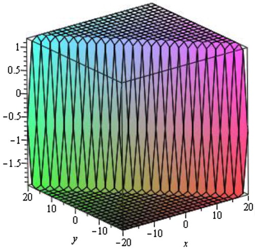
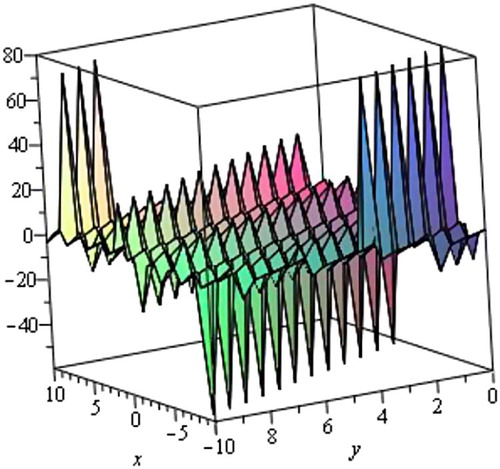
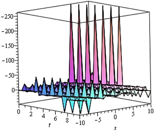
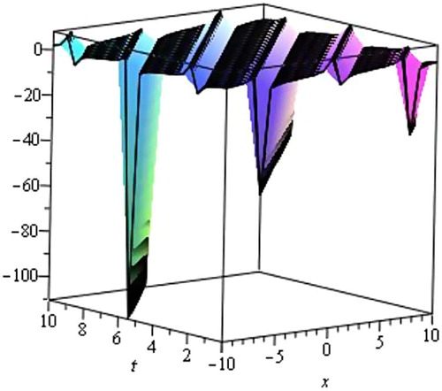
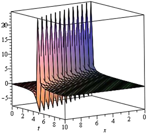
Graphical representation of the solutions:

The graphical illustrations of the solutions are given below in the figures with the aid of Maple (Figs. 1–^{Fig. 2Fig. 3Fig. 4}5).

Fig. 1 Kink wave solution $u_1\left(\eta \right)$ when $a_2=1,a_0=2,y=0,\lambda =3,\mu =2,c_1=1$.

Fig. 2 Singular Kink wave solution $u_2\left(\eta \right)$ when $a_2=10,a_0=8,y=0,\lambda =7,\mu =5,c_1=-10$.

Fig. 3 Singular Kink wave solution $u_3\left(\eta \right)$ when $a_2=1,a_0=2,y=0,\lambda =1,c_1=-1$.

Fig. 4 Singular Kink wave solution$u_4\left(\eta \right)$ when $a_2=3,a_0=2,y=0,\lambda =5,\mu =4,c_1=-2$.

Fig. 5 Singular Kink wave solution $u_5\left(\eta \right)$ when $a_2=0.5,a_0=0.2,y=0,\lambda =0.1,c_1=-0.1$.

3.2 Simplified Modified form of Camassa–Holm equation

Let us consider Simplified Modified form of Camassa–Holm equation.(17) $u_t+2\beta u_x-u_{xxt}+\delta u^2{u}_x=0,$(17)

where β and δ are some nonzero parameters.

We utilize the traveling wave variable$u\left(x,t\right)=u\left(\eta \right)$, η = x − Vt, we can convert Eq. (17)(17) $u_t+2\beta u_x-u_{xxt}+\delta u^2{u}_x=0,$(17) into an ordinary differential equation.(18) $-V{u}^{\prime }+2\beta u^{\prime }+V{u}^{‴}+\delta u^2{u}^{\prime }=0,$(18)

where the prime denotes the derivative with respect to η.

Now integrating Eq. (18)(18) $-V{u}^{\prime }+2\beta u^{\prime }+V{u}^{‴}+\delta u^2{u}^{\prime }=0,$(18) we have,(19) $-Vu+2\beta u+u^{″}V+\frac{1}{3}\delta u^3+C=0,$(19)

Balancing the u' and u² by using homogenous principal, we have$3M=M+2,$$M=1.$

Then the trial solution of Eq. (18)(18) $-V{u}^{\prime }+2\beta u^{\prime }+V{u}^{‴}+\delta u^2{u}^{\prime }=0,$(18) can be expressed as follows,(20) $u\left(\eta \right)={\alpha }_1\left(\exp \left(-\phi \left(\eta \right)\right)\right)+{\alpha }_0\text{},$(20)

where α₁ ≠ 0, α₀ is a constant to determined, while λ, µ are arbitrary constants.

Substituting $u,u^{\prime },u^{″},u^2$ into Eq. (19)(19) $-Vu+2\beta u+u^{″}V+\frac{1}{3}\delta u^3+C=0,$(19) and then equating the coefficients of $exp\left(-\phi \left(\eta \right)\right)$ to zero, we get(21) $\begin{array}{c}\frac{1}{3}\delta a_0^3+2a_0\beta +C+V{a}_1\mu \lambda -V{a}_0=0,\\ 2V{a}_1\mu +\delta a_0^2{a}_1+2a_1\beta +C+V{a}_1{\lambda }^2-V{a}_1=0,\\ \delta a_0{a}_1^2+3V{a}_1\lambda =0,\\ \frac{1}{3}\delta a_1^3+2V{a}_1=0\end{array}$(21)

Solving the set of algebraic equations, we obtain the following solution.$\{\lambda =\frac{1}{3}\frac{a_0\sqrt{-6\delta V}}{V},\mu =\frac{1}{6}\frac{3V-6\beta -\delta a_0^2}{V},{\text{a}}_1=-\frac{\sqrt{-6\delta V}}{\delta },\mathrm{C}=0,$

where λ and µ are arbitrary constants.

Now substituting the values into Eq. (20)(20) $u\left(\eta \right)={\alpha }_1\left(\exp \left(-\phi \left(\eta \right)\right)\right)+{\alpha }_0\text{},$(20) , we obtain,(22) $u=-\frac{-\delta a_0+\sqrt{6}\sqrt{–\delta V}{e}^{-\phi \left(\eta \right)}}{\delta }$(22)

Where η = x − Vt.

Now substituting Eq. (6)(6) $\phi \left(\eta \right)=\ln \left\{\frac{1}{2\mu }\left(-\sqrt{{\lambda }^2-4\mu }\tanh \left(\frac{\sqrt{{\lambda }^2-4\mu }}{2}\left(\eta +c_1\right)\right)-\lambda \right)\right\},$(6) to Eq. (10)(10) $\phi \left(\xi \right)=\ln \left(\eta +c_1\right)$(10) into Eq. (22)(22) $u=-\frac{-\delta a_0+\sqrt{6}\sqrt{–\delta V}{e}^{-\phi \left(\eta \right)}}{\delta }$(22) respectively, we get the following five traveling wave solutions of the Simplified Modified form of Camassa–Holm equation.

Case 1

When λ² − 4µ > 0 and µ ≠ 0, we obtain the hyperbolic function traveling wave solution.$u_1\left(\eta \right)=a_0-\frac{2\sqrt{6}\mu }{\left(-\sqrt{{\lambda }^2-4\mu }\tanh \left(\frac{\sqrt{{\lambda }^2-4\mu }}{2}\left(\eta +c_1\right)\right)-\lambda \right)},$

where η = x − Vt and where c₁ is an arbitrary constant.

Case 2

When λ² − 4µ < 0 and µ ≠ 0, we obtain trigonometric solution.$u_2\left(\eta \right)=a_0-\frac{2\sqrt{6}\mu }{\left(+\sqrt{-{\lambda }^2+4\mu }\tan \left(\frac{\sqrt{-{\lambda }^2+4\mu }}{2}\left(\eta +c_1\right)\right)-\lambda \right)},$

where η = x − Vt and where c₁ is an arbitrary constant.

Case 3

When µ = 0 and λ ≠ 0, we obtain exponential solution.$u_3\left(\eta \right)=a_0-\frac{\sqrt{6}\lambda }{exp\left({\left(\eta +c_1\right)}^{\lambda }-1\right)},$

where η = x − Vt and where c₁ is an arbitrary constant.

Case 4

When ${\lambda }^2-4\mu =0,\lambda \ne 0$, and µ ≠ 0, we obtain rational function solution.$u_4\left(\eta \right)=a_0-\frac{\sqrt{6}\left(\eta +c_1\right){\lambda }^2}{\left(2{\left(\eta +c_1\right)}^{\lambda }+2\right)},$

where η = x − Vt and where c₁ is an arbitrary constant.

Case 5

when λ = 0, and µ = 0, we obtain rational function solution.$u_5\left(\eta \right)=a_0-\frac{\sqrt{6}}{\left(\eta +c_1\right)},$

where η = x − Vt and where c₁ is an arbitrary constant.

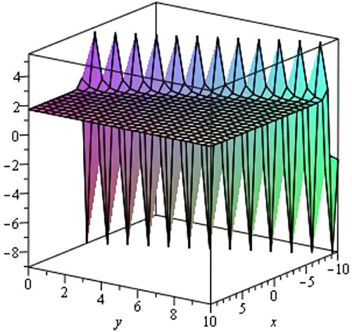
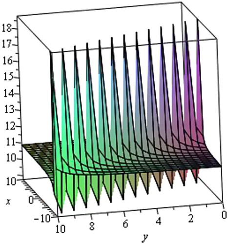
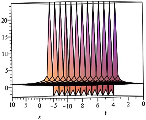
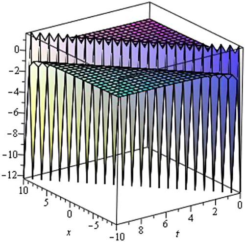
Graphical representation of the solutions:

The graphical illustrations of the solutions are given below in the figures with the aid of Maple (Figs. 6–^{Fig. 7Fig. 8Fig. 9}10).

Fig. 6 Kink wave solution $u_1\left(\eta \right)$ when $C=1,a_0=0.1,y=0,\lambda =0.2,\mu =0.5,c_1=-0.3$.

Fig. 7 Periodic solution $u_2\left(\eta \right)$ when $a_0=1,C=1,y=0,\lambda =0.1,\mu =0.2,c_1=-0.1$.

Fig. 8 Singular Kink wave solution $u_3\left(\eta \right)$ when $\mu =0.1,C=1,y=0,\lambda =0.3,a_0=0.1,c_1=-0.1$.

Fig. 9 Singular Kink wave solution $u_4\left(\eta \right)$ when $a_0=0.1,C=1,y=0,\lambda =0.1,\mu =1,c_1=-0.1$.

Fig. 10 Singular Kink wave solution $u_5\left(\eta \right)$ when $C=1,y=0,\mu =0.1,a_0=0.1,c_1=-0.1$.

Conclusions: The $\exp \left(-\phi \left(\eta \right)\right)$-expansion method is very important in finding the exact solutions of nonlinear evolution equations. In this article, we have successfully formulated the exact and traveling wave solutions to the generalized Zakharov–Kuznetsov–Benjamin–Bona–Mahony equation and Simplified Modified form of Camassa–Holm equation. The wave solutions are obtained through the hyperbolic, trigonometric, exponential and rational functions. The calculation procedure is simple, direct and constructive. This study shows that the method is quite efficient and much effective for finding exact solutions of nonlinear evolution equations (NLEEs). Also, we observe that the method is straightforward and can be applied to many other nonlinear evolution equations.