Numerical solution of quadratic Riccati differential equations

Abstract

The quadratic Riccati differential equations are part of non-linear differential equations which have many applications. This paper introduces the classical fourth order Runge Kutta method (RK4) for solving the numerical solution of the quadratic Riccati differential equations. To validate the applicability of the method on the proposed equation, some model examples have been solved for different values of mesh sizes. The numerical results in terms of point wise absolute errors presented in tables and graphs show that the present method approximates the exact solution very well.

Keywords:

• Riccati differential equation
• Runge Kutta method

1 Introduction

The Riccati differential equation is a well-known non linear differential equation and has different applications in engineering and science domains, such as robust stabilization, stochastic realization theory, network synthesis, optimal control and in financial mathematics [1]. Non linear deferential equations are essential tools for modeling many physical situations, for instance, spring mass systems, resistor–capacitor–induction circuits, bending of beams, chemical reaction, pendulums, the motion of rotating mass around body and so on [2].

Thus, the problem has attracted much attention and has been studied by many authors. Recently, various methods are used like: using the method of Bezier curves, by developing the Bezier polynomial of degree n [3], the multistage variational iteration method is applied as a new efficient method for solving quadratic Riccati differential equation [4], using Legendre scaling functions consisting of expanding the required approximate solution as the elements of Legendre scaling functions and the operational matrix of integral, then reducing the problem to a set of algebraic equations [5] and approximate solution of generalized Riccati differential equations by iterative decomposition algorithm [6]. The solution of Riccati equation with variable co-efficient by differential transformation method (DTM) [7] has presented the absolute error between the approximated solutions which are obtained by DTM.

However, the above mentioned methods have some restrictions and disadvantages. For instance, there is a big difference between the results obtained by DTM, but as we have shown in examples there is a small point wise absolute error between the numerical result obtained by RK4 and the exact value. The classical RK4 is widely used for solving initial value problems and provides approximations which converge to the true solution as h approaches zero [8,9].

In this paper, we introduce classical RK4 method for solving the nonlinear Riccati quadratic differential equation. The stability of the method for the problem under consideration has also been investigated. The approximate solution obtained by the proposed method versus the exact solution for different values of mesh size on some nodal points has been given. To validate the efficiency of the method, four model examples are solved.

2 Formulation of the method

Consider the quadratic Riccati differential equation of the form:(1) $\frac{dy}{dt}=p\left(t\right)+q\left(t\right)y+r\left(t\right)y^2$(1) with initial value condition(2) $y\left(t_0\right)=\alpha$(2) where $p\left(t\right),q\left(t\right)$, $r\left(t\right)$ are continuous with $r\left(t\right)\ne 0$, and $t_0\text{},\alpha$ are arbitrary constants for $y\left(t\right)$, which is an unknown function. To describe the scheme, we denote the problem in Eq. (1)(1) $\frac{dy}{dt}=p\left(t\right)+q\left(t\right)y+r\left(t\right)y^2$(1) as:(3) $\frac{dy}{dt}=f\left(t,y\right)$(3) and divide the interval $\left[t_0\text{},t_f\right]$ into N equal subintervals of mesh length h and the mesh points given by $t_i=t_0+ih$;$i=1,2,\dots n$. To solve the problem, we apply the single step method that requires information about the solution at $t_i$ to calculate $t_{i+1}$ [8]. Let the general numerical solution of Eq. (1)(1) $\frac{dy}{dt}=p\left(t\right)+q\left(t\right)y+r\left(t\right)y^2$(1) be given as:(4) $y_{i+1}=y_i+{\displaystyle \sum _{i=1}^4{w}_i{k}_i}$(4) where(5) $k_i=hf\left(t_i+c_{i}h,y_i+{\displaystyle \sum _{j=1}^3{a}_{ij}{k}_j}\right),\text{for}i=1,2,3,4$(5) and the parameters $c_i,a_{ij}\text{for}i=2,3,4$; and $w_1\text{},\dots ,w_4$ are chosen in such a way that the numerical solution $y_{i+1}$ approximates the exact solution $y\left(t_{i+1}\right)$of Eq. (1)(1) $\frac{dy}{dt}=p\left(t\right)+q\left(t\right)y+r\left(t\right)y^2$(1) very well.

Now, expanding $k_2\text{},k_3\text{},k_4$ in Taylor series about $t_i$, substituting in Eq. (4)(4) $y_{i+1}=y_i+{\displaystyle \sum _{i=1}^4{w}_i{k}_i}$(4) and matching the coefficients of $h,h^2\text{},h^3\text{and}{h}^4$, we obtain the systems of equations which on solving gives us:$\begin{array}{l}{c}_2=c_3=1/2,c_4=1,w_2=w_3=1/3,w_1=w_4=1/6,\\ a_{21}=1/2,a_{31}=0,a_{32}=1/2,a_{41}=a_{42}=0,a_{43}=1.\end{array}$

Thus, Eq. (4)(4) $y_{i+1}=y_i+{\displaystyle \sum _{i=1}^4{w}_i{k}_i}$(4) becomes an explicit classical fourth order Runge Kutta method and written as:(6) $y_{i+1}=y_i+\frac{1}{6}\left(k_1+2k_2+2k_3+k_4\right)$(6) where$\begin{array}{l}{k}_1=hf\left(t_i\text{},y_y\right)\\ k_2=hf\left(t_i+\frac{h}{2},y_i+\frac{k_1}{2}\right)\\ k_3=hf\left(t_i+\frac{h}{2},y_i+\frac{k_2}{2}\right)\\ k_4=hf\left(t_i+h,y_i+k_3\right)\end{array}$

In the determination of the parameters, since the terms up to $O\left(h^4\right)$ are compared, the truncation error is $O\left(h^5\right)$ and the order of the method is 4.

3 Stability and convergence analysis

Consider Eq. (1)(1) $\frac{dy}{dt}=p\left(t\right)+q\left(t\right)y+r\left(t\right)y^2$(1) at the discretized point as:(7) $f\left(t_i\text{},y_i\right)=p\left(t_i\right)+q\left(t_i\right)y\left(t_i\right)+r\left(t_i\right)y^2\left(t_i\right)$(7)

Further, consider the linear first order test differential equation:$y^{\prime }=\lambda y,y\left(t_0\right)=y_0$Where $\lambda$ is a constant, and has its solution in the form of$y\left(t\right)=y\left(t_0\right)e^{\left(\lambda \left(t-t_0\right)\right)}\text{which}\text{at}t=t_0+nh.$

The solution becomes:(8) $y\left(t_n\right)=y\left(t_0\right)e^{\lambda nh}=y_0{\left(e^{\lambda h}\right)}^n$(8)

Let the non-linear quadratic Riccati differential equation of the form given in Eqs. (1)–(3) and Eq. (7)(7) $f\left(t_i\text{},y_i\right)=p\left(t_i\right)+q\left(t_i\right)y\left(t_i\right)+r\left(t_i\right)y^2\left(t_i\right)$(7) written as:(9) $y\prime =f\left(t,y\right);y\left(t_0\right)=y_0=\alpha$(9)

The non-linear function Eq. (9)(9) $y\prime =f\left(t,y\right);y\left(t_0\right)=y_0=\alpha$(9) can be linearized by expanding the function in Taylor series about the point $\left(t_0\text{},y_0\right)$ and truncating it after the first term:(10) $y^{\prime }=f\left(t_0\text{},y_0\right)+\left(t-t_0\right)\frac{\partial f}{\partial t}\left(t_0\text{},y_0\right)+\left(y-y_0\right)\frac{\partial f}{\partial y}\left(t_0\text{},y_0\right)$(10)

Using Eq. (7)(7) $f\left(t_i\text{},y_i\right)=p\left(t_i\right)+q\left(t_i\right)y\left(t_i\right)+r\left(t_i\right)y^2\left(t_i\right)$(7) and by the chain rule differentiation, we have $y^{\prime }=p_0+q_0{y}_0+r_0{y}_0^2+\left(t-t_0\right)[p_0^{\prime }+q_0^{\prime }{y}_0+q_0{y}_0^{\prime }+r_0^{\prime }{y}_0^2+2r_0{y}_0{y}_0^{\prime }]+y[q_0+2r_0{y}_0{y}_0^{\prime }]-q_0{y}_0-2r_0{y}_0^2{y}_0^{\prime }$ For simplicity, consider $p\left(t_0\right)=p_0\text{},q\left(t_0\right)=q_0\text{},r\left(t_0\right)=r_0\text{},y\left(t_0\right)=y_0\text{},y^{\prime }\left(t_0\right)=y_0^{\prime }$ and using Eq. (2)(2) $y\left(t_0\right)=\alpha$(2) $y\left(t_0\right)=y_0=\alpha =\text{constant}$; Thus, $y_0^{\prime }=0$.(11) $\Rightarrow y^{\prime }=q_{0}y+p_0+r_0{y}_0^2+\left(t-t_0\right)[p_0^{\prime }+q_0^{\prime }{y}_0+r_0^{\prime }{y}_0^2]$(11)

This can be written as:(12) $y^{\prime }=\lambda y+c$(12) where $\lambda =q_0\text{},c=p_0+r_0{y}_0^2+\left(t-t_0\right)[p_0^{\prime }+q_0^{\prime }{y}_0+r_0^{\prime }{y}_0^2]$

Dividing both sides of Eq. (12)(12) $y^{\prime }=\lambda y+c$(12) by $\lambda$, we obtain $\frac{y^{\prime }}{\lambda }=y+\frac{c}{\lambda }$.

If $w=y+\frac{c}{\lambda }$, then we have:(13) $y=w-\frac{c}{\lambda }$(13)

Substituting Eq. (13)(13) $y=w-\frac{c}{\lambda }$(13) into Eq. (12)(12) $y^{\prime }=\lambda y+c$(12) gives:(14) $w^{\prime }=\lambda w$(14) which is called the linear test equation for the non-linear Eq. (1)(1) $\frac{dy}{dt}=p\left(t\right)+q\left(t\right)y+r\left(t\right)y^2$(1) .

The solution of this test equation, Eq. (15)(15) $w=k{e}^{\lambda t}$(15) , is:(15) $w=k{e}^{\lambda t}$(15)

Now, by considering Eq. (6)(6) $y_{i+1}=y_i+\frac{1}{6}\left(k_1+2k_2+2k_3+k_4\right)$(6) , we have:$\begin{array}{c}{k}_1=hf\left(t_n\text{},y_n\right)=\lambda h{y}_n\\ k_2=\lambda h{y}_n+\frac{1}{2}{\left(\lambda h\right)}^2{y}_n=\left[\lambda h+\frac{{\left(\lambda h\right)}^2}{2}\right]y_n\\ k_3=\lambda h{y}_n+\frac{1}{2}\lambda h\left[\lambda h+\frac{1}{2}{\left(\lambda h\right)}^2\right]y_n=\left[\lambda h+\frac{{\left(\lambda h\right)}^2}{2}+\frac{{\left(\lambda h\right)}^3}{4}\right]y_n\\ k_4=\lambda h{y}_n+\lambda h\left[\lambda h+\frac{{\left(\lambda h\right)}^2}{2}+\frac{{\left(\lambda h\right)}^3}{4}\right]y_n\\ =\left[\lambda h+{\left(\lambda h\right)}^2+\frac{{\left(\lambda h\right)}^3}{2}+\frac{{\left(\lambda h\right)}^4}{4}\right]y_n\end{array}$

On substituting the values for $k_1\text{},k_2\text{},k_{3}and{k}_4$, we obtain:$\begin{array}{c}{y}_{n+1}=y_n+\frac{1}{6}\lambda h{y}_n+\frac{1}{3}\left[\left(\lambda h+\frac{{\left(\lambda h\right)}^2}{2}\right)y_n\right]\\ +\frac{1}{3}\left[\left(\lambda h+\frac{{\left(\lambda h\right)}^2}{2}+\frac{{\left(\lambda h\right)}^3}{4}\right)y_n\right]\\ +\frac{1}{6}\left[\left(\lambda h+{\left(\lambda h\right)}^2+\frac{{\left(\lambda h\right)}^3}{2}+\frac{{\left(\lambda h\right)}^4}{4}\right)y_n\right]\end{array}$$\Rightarrow y_{n+1}=\left[1+\lambda h+\frac{{\left(\lambda h\right)}^2}{2}+\frac{{\left(\lambda h\right)}^3}{6}+\frac{{\left(\lambda h\right)}^4}{24}\right]y_n$(16) $y_{n+1}=E\left(\lambda h\right)y_n$(16) Where $E\left(\lambda h\right)=1+\lambda h+\frac{{\left(\lambda h\right)}^2}{2}+\frac{{\left(\lambda h\right)}^3}{6}+\frac{{\left(\lambda h\right)}^4}{24}$

From Eq. (8)(8) $y\left(t_n\right)=y\left(t_0\right)e^{\lambda nh}=y_0{\left(e^{\lambda h}\right)}^n$(8) , it is easily observed that the exact value of $y\left(t_n\right)$ increases for the constant $\lambda >0$ and decreases for $\lambda <0$ with the factor $e^{\lambda h}$. While from Eq. (16)(16) $y_{n+1}=E\left(\lambda h\right)y_n$(16) the approximate value of $y_n$increases or decreases with the factor of $E\left(\lambda h\right)$. If $\lambda h>0$, then $e^{\lambda h}\ge 1$, so the fourth order RK method is relatively stable. If $\lambda h<0$, then the interval of absolutely stable is $-2.78<\lambda h<0$.

The computational rate of convergence can also be obtained by using the double mesh principle defined below. Consider the numerical solution obtained by Eq. (6)(6) $y_{i+1}=y_i+\frac{1}{6}\left(k_1+2k_2+2k_3+k_4\right)$(6) and let $Z_h=\max \left|y_i^h-y_i^{h/2}\right|,i=1,2,\dots ,N-1$. Where $y_i^h$ is the numerical solution on the mesh ${\left\{t_i\right\}}_1^{N-1}$ at the nodal point $t_i=t_0+ih,i=1,2,\dots ,N-1$ and where $y_i^{h/2}$ is the numerical solution at the nodal point t₁ on the mesh ${\left\{t_i\right\}}_1^{2N-1}$ where, $t_i=t_0+ih/2,i=1,2,\dots ,2N-1$.

In the same way one can define $Z_{h/2}$ by replacing $h$ by $h/2$ and $N-1$ by $2N-1$, that is, $Z_{h/2}=\max \left|y_i^{h/2}-y_i^{h/4}\right|,i=1,2,\dots ,2N-1$.

The computed rate of convergence is defined as:(17) $\text{Rate}=\frac{\log Z_h-\log Z_{h/2}}{\log 2}$(17)

Numerical examples are given to illustrate the efficiency and convergence of this method.

In Table 1, the rate of convergence for examples 2, 3 and 4 respectively is given at different mesh sizes.

Table 1 Rate of convergence for some model examples with different mesh sizes.

	N	10	40	70	100	200	400
Rate of convergence	Example 2	3.9522	3.9851	3.9915	3.9941	3.9972	3.9935
	Example 3	3.9584	3.9904	3.9946	3.9964	4.0010	4.0581
	Example 4	4.1313	4.0350	4.0202	4.0144	4.0076	3.9293

4 Numerical examples

To validate the applicability of the method, four quadratic Riccati differential equations have been considered. For each N, the point wise absolute errors are approximated by the formula, $\Vert E\Vert =\left|y\left(t_i\right)-y_i\right|$, for $i=0,1,2,\dots N$ and where,$y\left(t_i\right)$ and $y_i$ are the exact and computed approximate solution of the given problem respectively, at the nodal point $t_i$.

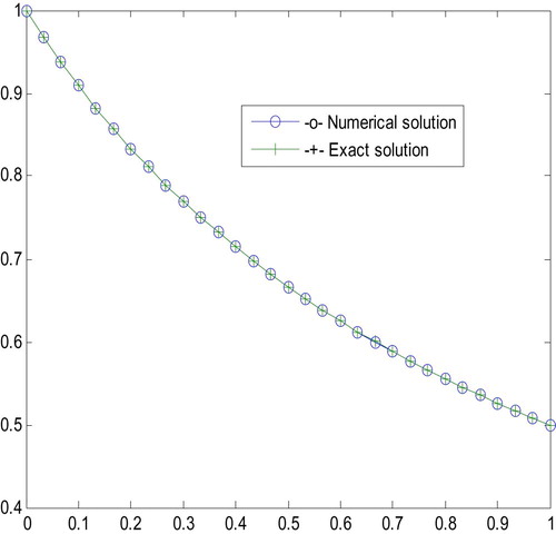
Example 1

Consider the following quadratic Riccati differential equation [3]

$\begin{array}{l}{y}^{\prime }\left(t\right)=16t^2-5+8ty\left(t\right)+y^2\left(t\right),0\le t\le 1\\ y\left(0\right)=1\end{array}$where the exact solution is: $y\left(t\right)=1-4t$.

The numerical solution in terms of point wise absolute errors by the comparing with the previous method is given in Table 2.

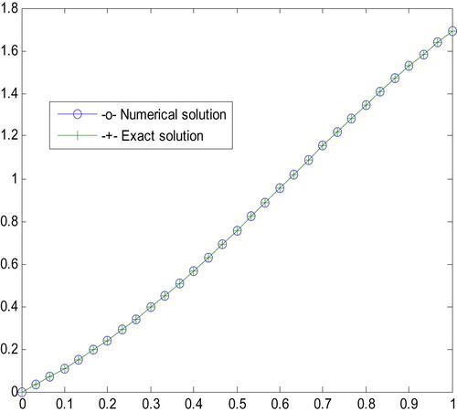
Example 2

Consider the following quadratic Riccati differential equation [3–^[4][5]6]

$\begin{array}{l}{y}^{\prime }\left(t\right)=1+2y\left(t\right)-y^2\left(t\right),0\le t\le 1\\ y\left(0\right)=0,\end{array}$where the exact solution is: $y\left(t\right)=1+\sqrt{2}\tanh \left(\sqrt{2}t+0.5\ln \left(\frac{\sqrt{2}-1}{\sqrt{2}+1}\right)\right)$.

Table 2 Absolute error for example 1 (mesh size $h=0.1$ OR N = 10).

t	Method [3]	The present method
0.0	0.0000000000000	0
0.1	0.000233600365141	0
0.3	0.00045422294912	2.2204e-16
0.5	9.375e-11	2.2204e-16
0.7	0.00045422275331	2.2204e-16
0.9	0.00023360043610	4.4409e-16
1.0	0.0000000000000	8.8818e-16

The numerical solution in terms of absolute errors is given in Table 3.

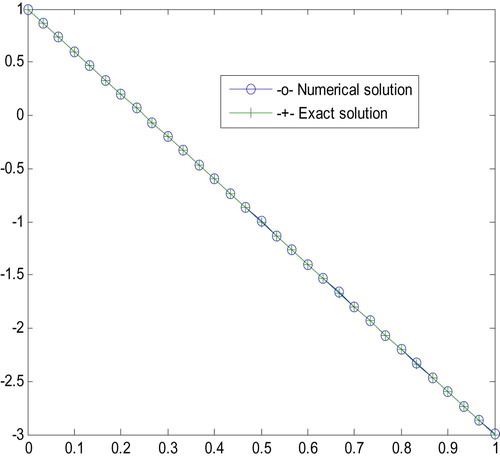
Example 3

Consider the following quadratic Riccati differential equation [3]

$\begin{array}{l}{y}^{\prime }\left(t\right)=e^t-e^{3t}+2e^{2t}y\left(t\right)-e^t{y}^2\left(t\right),0\le t\le 1\\ y\left(0\right)=1.\end{array}$where the exact solution is $y\left(t\right)=e^t$.

Table 3 Absolute error for example 2.

t	N = 10	N = 40	N = 70	N = 100	N = 200	N = 400
0.1	2.2551e-06	9.8491e-09	1.0669e-09	2.8533e-10	1.6233e-11	1.0184e-12
0.2	4.7763e-06	2.0641e-08	2.2327e-09	5.3915e-10	3.3923e-11	2.1275e-12
0.3	7.3083e-06	3.1235e-08	3.3731e-09	8.1402e-10	5.1180e-11	3.2087e-12
0.4	9.5635e-06	4.0441e-08	4.3607e-09	1.0517e-09	6.6078e-11	4.1415e-12
0.5	1.1301e-05	4.7374e-08	5.1021e-09	1.2299e-09	7.7230e-11	4.8390e-12
0.6	1.2408e-05	5.1724e-08	5.5661e-09	1.3414e-09	8.4199e-11	5.2707e-12
0.7	1.2940e-05	5.3815e-08	5.7892e-09	1.3949e-09	8.7546e-11	5.4756e-12
0.8	1.3100e-05	5.4419e-08	5.8528e-09	1.4101e-09	8.8489e-11	5.5316e-12
0.9	1.3141e-05	5.4381e-08	5.8450e-09	1.4079e-09	8.8322e-11	5.5178e-12
1	1.3245e-05	5.4260e-08	5.8236e-09	1.4019e-09	8.7889e-11	5.5029e-12

The numerical solution in terms of absolute errors is given in Table 4.

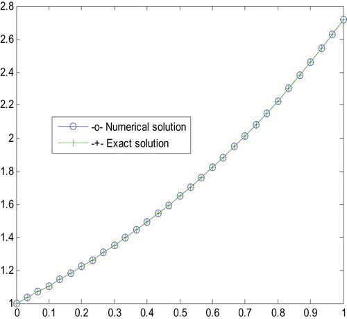
Example 4

Consider the following Riccati differential equation [5]

$\begin{array}{l}{y}^{\prime }\left(t\right)=\frac{-1}{1+t}+y\left(t\right)-y^2\left(t\right),0\le t\le 1\\ y\left(0\right)=1\end{array}$with analytic solution $y\left(t\right)=\frac{1}{1+t}$. Table 5 shows that the numerical solution in terms of absolute error for different step size h.

Table 4 Absolute errors for example 3.

t	N = 10	N = 40	N = 70	N = 100	N = 200	N = 400
0.1	1.1153e-07	4.5427e-10	4.8711e-11	1.1722e-11	7.3475e-13	4.5963e-14
0.2	2.6297e-07	1.0710e-09	1.1484e-10	2.7633e-11	1.7317e-12	1.0880e-13
0.3	4.6838e-07	1.9073e-09	2.0451e-10	4.9211e-11	3.0835e-12	1.9384e-13
0.4	7.4674e-07	3.0404e-09	3.2600e-10	7.8447e-11	4.9163e-12	3.0909e-13
0.5	1.1237e-06	4.5748e-09	4.9051e-10	1.1803e-10	7.3965e-12	4.6496e-13
0.6	1.6338e-06	6.6511e-09	7.1312e-10	1.7160e-10	1.0753e-11	6.7191e-13
0.7	2.3239e-06	9.4596e-09	1.0142e-09	2.4406e-10	1.5293e-11	9.5124e-13
0.8	3.2569e-06	1.3257e-08	1.4214e-09	3.4203e-10	2.1432e-11	1.3305e-12
0.9	4.5182e-06	1.8390e-08	1.9717e-09	4.7445e-10	2.9730e-11	1.8439e-12
1	6.2225e-06	2.5327e-08	2.7154e-09	6.5340e-10	4.0941e-11	2.5673e-12

Table 5 Absolute errors for example 4.

t	N = 10	N = 40	N = 70	N = 100	N = 200	N = 400
0.1	3.8296e-07	1.2712e-09	1.3226e-10	3.1445e-11	1.9426e-12	1.2057e-13
0.2	5.7951e-07	1.9396e-09	2.0206e-10	4.8062e-11	2.9710e-12	1.8452e-13
0.3	6.8133e-07	2.2939e-09	2.3918e-10	5.6914e-11	3.5196e-12	2.1860e-13
0.4	7.3394e-07	2.4816e-09	2.5893e-10	6.1630e-11	3.8125e-12	1.8452e-13
0.5	7.6091e-07	2.5808e-09	2.6941e-10	6.4137e-11	3.9686e-12	2.4647e-13
0.6	7.7483e-07	2.6340e-09	2.7506e-10	6.5490e-11	4.0530e-12	2.5280e-13
0.7	7.8257e-07	2.6648e-09	2.7834e-10	6.6278e-11	4.1022e-12	2.5668e-13
0.8	7.8799e-07	2.6865e-09	2.8066e-10	6.6837e-11	4.1374e-12	2.5946e-13
0.9	7.9326e-07	2.7069e-09	2.8284e-10	6.7358e-11	4.1697e-12	2.6190e-13
1	7.9961e-07	2.7304e-09	2.8533e-10	6.7954e-11	4.2070e-12	2.6240e-13

5 Numerical results

The following graphs (Figs. 1–^{Fig. 2Fig. 3}4) show the numerical solutions obtained by the present method versus its corresponding exact solution.

Fig. 1 The graph of numerical and exact solution of example 1 for N = 30.

Fig. 2 The graph of numerical and exact solution of example 2 for N = 30.

Fig. 3 The graph of numerical and exact solution of example 3 for N = 30.

Fig. 4 The graph of numerical and solution exact solution of example 4 for N = 30.

6 Discussion and conclusion

In this paper, we presented classical KR4 for solving quadratic Riccati differential equations. To further collaborate the applicability of the proposed method; tables of point wise absolute error and graphs have been plotted for examples 1–4 for exact solution versus the numerical solutions at different values of mesh size h. Table 2 shows that the absolute errors obtained by RK4 have been compared with absolute errors obtained by Ref. [3]. Tables 3–^{Table 4}5 also show that the point wise absolute error decreases as the mesh size h decreases, which in turn shows the convergence of the computed solution. Generally, the present method is computationally: stable, effective, simple to use, convergent and give accurate solution than some previously existing methods, including the more recent method in Ref. [3].