A computational method for solving a class of singular boundary value problems arising in science and engineering

Abstract

This note deals with a new computational method for solving a class of singular boundary value problems. The method is based upon Bernstein Polynomials. The properties of Bernstein Polynomials, together with Bernstein operational matrix for differentiation formula, are presented and utilized to reduce the given singular boundary value problems to the set of algebraic equations. The proposed method is applied to solve some test problems with the comparison between the computational solutions and the exact solutions. The results indicate that the proposed algorithm provides high reliability and good accuracy.

Keywords:

• Computational method
• Bernstein operational matrices
• Nonlinear differential equations
• Singular boundary value problems

1 Introduction

In this paper, we consider the class of singular boundary value problems (SBVPs) of the form(1) $y^{″}\left(x\right)+\frac{\alpha }{x}{y}^{\prime }\left(x\right)+p\left(x\right)y\left(x\right)=r\left(x\right),0<x\le 1and\alpha >0$(1) with the boundary conditions(2) $y\left(0\right)=a_1\text{},y\left(1\right)=b\left(\text{or}\right)y^{\prime }\left(0\right)=a_2\text{},y\left(1\right)=b$(2) where $p\left(x\right)$ and $r\left(x\right)$ are analytic in $x\in \left(0,1\right)$ and $a_1\text{},a_2\text{},b$ and $\alpha$ are finite constants. Problem (1) has singularity at the initial point $x=0$. We note that the main difficulty arises in the singularity of the equations at $x=0$.

The numerical treatment of singular boundary value problems has always been a difficult and challenging task due to the singular behavior that occurs at a point.

In recent years, strenuous action and interest have been investigating singular boundary value problems (SBVPs) and a number of methods have been proposed. The singular boundary value problems arise frequently in many branches of applied mathematics, mechanics, nuclear physics, atomic theory and chemical sciences. Hence, the singular boundary value problems have attracted much attention and have been investigated by many researchers. Kadalbajoo and Agarwal treated the homogeneous equation using Chebyshev polynomial and B-spline [1]. Kanth and Reddy solved a particular singular boundary value problem by applying higher order finite difference method [2].The same authors investigated by using the cubic spline [3] method. Mohanty et al. [4] introduced accurate cubic spline method for solving the singular boundary value problems. Variational iteration method (VIM) was introduced by Wazwaz [5] for solving nonlinear singular boundary value problems.

The authors [6,7] elaborately discussed singular boundary value problems and solved by the methods based on reproducing kernel space. Galerkin and Collocation methods are presented for solving two-point boundary value problems by Mohsen and El-Gamel [8]. Secer and Kurulay [9] described the Sinc-Galerkin method for singular Dirichlet-type boundary value problems. Rashidinia et al. [10] proposed a reliable parametric spline method.

The purpose of this note is to develop a reliable operational matrix method for singular boundary value problems. The aim of the present paper is to apply Bernstein operational matrix of differentiation to propose a reliable numerical technique for solving SBVPs.

With the advent of computer graphics, Bernstein polynomial restricted to the interval $x\in \left[0,1\right]$becomes important in the form of Bezier curves [11,12]. Bernstein polynomials have many constructive properties such as the positivity, the continuity, recursive relation, symmetry and unity partition of the basis set over the interval. For this reason, Bernstein operational matrix method is a new and rising area in applied mathematical research which has gained considerable attention in dealing with differential equations. Optimal stability of the Bernstein basis was discussed by Farouki and Goodman [13]. Bhatta and Bhatti [14] have been used modified Bernstein polynomials for solving Korteweg-de Vries (KdV) equation. Chakrabarti and Martha [15] described a method for Fredholm integral equations. Bhattacharya and Mandal [16] presented Bernstein polynomials method for Volterra integral equations. Yousefi and Behroozifar [17] found the operational matrices of integration and product of B-polynomials. The same authors [18] introduced the Bernstein operational matrix method (BOMM) for solving the parabolic type partial differential equations (PDEs). Isik et al. [19] have demonstrated a new method to solve high order linear differential equations with initial and boundary conditions. Ordokhani et al. [20] introduced Bernstein polynomial for solving differential equations. Singh et al. [21] established the Bernstein operational matrix of integration for solving differential equations. Doha et al. [22,23] have implemented and proved new formulas about derivatives and integrals of Bernstein polynomials and solving high even-order differential equations by Bernstein polynomial based method. Yousefi et al. [24] described the Ritz-Galerkin method for solving an initial boundary value problem that combines Neumann and integral condition for the wave equation. Bhattacharya et al. [25] implemented the algorithm for integro differential equations. Shen et al. [26] suggested a boundary knot method (BKM) to solve Helmholtz problems with boundary singularities. Lin et al. [27] used the efficient boundary knot method to obtain the solution of axisymmetric Helmholtz problems. Recently, Pirabaharan et al. [28] introduced a Bernstein operational matrix method for boundary value problems.

The objective of this paper is to give the computational method based on the Bernstein operational matrix for differentiation for the class of singular boundary value problems (SBVPs). The proposed algorithm converted to the given SBVP to the system of algebraic equations with unknown coefficients and are solved easily by using mathematical tool like MATLAB.

The outline of the paper is as follows. In section 2, we review the basic properties of Bernstein polynomials and we develop the Bernstein operational matrix for derivative. Section 3 implemented and presented the methods of solution for the singular boundary value problems. In Section 4, some numerical examples are presented to show the efficiency and the applicability of the suggested algorithm. Conclusion is given in Section 5.

2 Properties of Bernstein polynomials [29]

The Bernstein basis polynomials of degree n are defined in the interval (0, 1) as [17,18](3) $b_i^n\left(x\right)=\left(\begin{array}{l}n\\ i\end{array}\right)x^i{\left(1-x\right)}^{n-i}\text{},i=0,1,2,\dots ,n$(3)

These Bernstein polynomials form a complete basis on the interval (0, 1). Using the recursive definition to generate these polynomials$b_i^n\left(x\right)=\left(1-x\right)b_i^{n-1}\left(x\right)+x{b}_{i-1}^{n-1}\left(x\right),i=0,1,2,\dots ,n$where $b_{-1}^{n-1}\left(x\right)=0$ and $b_n^{n-1}\left(x\right)=0$.

Since the power basis forms a basis for the space of polynomials of degree less than or equal to n, any n^th degree Bernstein polynomial can be expressed in terms of the power basis. This can be computed by using the binomial expansion,(4) $\begin{array}{c}\text{one}\text{can}\text{illustrate}\text{that}{b}_i^n\left(x\right)={\displaystyle \sum _{j=1}^n{\left(-1\right)}^{j-1}\left(\begin{array}{c}n\\ i\end{array}\right)\left(\begin{array}{c}n-1\\ j-i\end{array}\right)x^j}\text{},\\ i=0,1,\dots ,n\end{array}$(4)

By using the property, the dual basis is defined as follows:${\displaystyle \underset{0}{\overset{1}{\int }}{b}_i^n\left(x\right)d_j^n\left(x\right)}=\{\begin{array}{ll}1,\hfill & i=j\hfill \\ \hfill & \begin{array}{cccc}& & for& i,j=0,1,2,\dots ,n\end{array}\hfill \\ 0,\hfill & i\ne j\hfill \end{array}.$

A function$f\left(x\right)$, square integrable in the interval [0, 1], may be written in terms of Bernstein basis [17,18].

Practically, only the first (n + 1) term Bernstein polynomials are considered.

Therefore, we can write(5) $f\left(x\right)\approx {\displaystyle \sum _{i=0}^n{c}_i{b}_i^n\left(x\right)}=C^{T}B\left(x\right)$(5) where the Bernstein coefficient vector $C$ and the Bernstein vector $B\left(x\right)$ is Bernstein vector are given by(6) $\begin{array}{c}{C}^T=\left[c_0\text{},c_1\text{},\dots ,c_n\right],\\ B\left(x\right)={\left[b_0^n\left(x\right),b_1^n\left(x\right),\dots ,b_n^n\left(x\right)\right]}^T\text{},\end{array}$(6) then$c_i={\displaystyle \underset{0}{\overset{1}{\int }}f\left(x\right)d_i^n\left(x\right)dx},i=0,1,2,\dots ,n.$

Jutler [30] has derived explicit representations,$d_j^n\left(x\right)={\displaystyle \sum _{k=0}^n{\lambda }_{jk}{b}_k^n\left(x\right)},j=0,1,2,\dots ,n$for the dual basis functions, defined by the coefficients(7) $\begin{array}{l}{\lambda }_{jk}=\frac{{\left(-1\right)}^{j+i}}{\left(\begin{array}{c}n\\ j\end{array}\right)\left(\begin{array}{c}n\\ k\end{array}\right)}{\displaystyle \sum _{i=0}^{\min \left(j\cdot k\right)}\left(2i+1\right)\left(\begin{array}{c}n+i+1\\ n-j\end{array}\right)\left(\begin{array}{c}n-i\\ n-j\end{array}\right)\left(\begin{array}{c}n+i+1\\ n-k\end{array}\right)\left(\begin{array}{c}n-i\\ n-k\end{array}\right)}\\ \text{for}j,k=0,1,2,\dots ,n.\end{array}$(7)

The Bernstein polynomials are useful for practical computations on account of its essential numerical stability [13]. One of the valuable property of Bernstein basis polynomials is that they all disappear at boundaries of the interval, except the first and the last one, which are equal to one at $x=0$ and $x=1$ respectively. This gives greater flexibility which imposes boundary conditions at the end points of the interval [31]. Also, Bernstein polynomials have two most important properties:

(i)	Unity partition property

${\displaystyle \sum _{i=0}^n{b}_i^n\left(x\right)=1},x\in \left[0,1\right],$

(ii)	Positivity property

$b_i^n\left(x\right)\ge 0,\text{for}i=0,1,2,\dots ,n.$$b_i^n\left(x\right)=0,\text{if}i<0\text{or}i>n$where $b_i^n\left(x\right)$ is the Bernstein polynomial of degree $n$.

2.1 The operational matrix of the derivative [29]

The derivative of the vector B(x) can be written as(8) $\frac{dB\left(x\right)}{dx}=D^{\left(1\right)}B\left(x\right)$(8) where $D^{\left(1\right)}$ is the operational matrix of derivative of $\left(n+1\right)\times \left(n+1\right)$ order and is specified in Ref. [17] as(9) $D^{\left(1\right)}=AVB*$(9) $\text{Here}A={\left[\begin{array}{cccccc}{\left(-1\right)}^0\left(\begin{array}{c}n\\ 0\end{array}\right)& {\left(-1\right)}^1\left(\begin{array}{c}n\\ 0\end{array}\right)\left(\begin{array}{c}n-0\\ 1\end{array}\right)& .& .& .& {\left(-1\right)}^{n-0}\left(\begin{array}{c}n\\ 0\end{array}\right)\left(\begin{array}{c}n-0\\ n-0\end{array}\right)\\ .& & & & & \\ & .& & & & \\ & & .& & & \\ 0& {\left(-1\right)}^0\left(\begin{array}{c}n\\ i\end{array}\right)& .& .& .& {\left(-1\right)}^{n-i}\left(\begin{array}{c}n\\ i\end{array}\right)\left(\begin{array}{c}n-i\\ n-i\end{array}\right)\\ .& & & & & \\ .& .& & & & \\ .& & .& & & \\ 0& .& .& .& 0& {\left(-1\right)}^0\left(\begin{array}{c}n\\ n\end{array}\right)\end{array}\right]}_{\left(n+1\right)\times \left(n+1\right)}$$V={\left[\begin{array}{ccccccc}0& 0& 0& .& .& .& 0\\ 1& 0& 0& .& .& .& 0\\ 0& 2& 0& .& .& .& 0\\ .& .& .& & .& & .\\ .& .& .& & .& & .\\ .& .& .& & .& & .\\ 0& 0& 0& .& .& .& n\end{array}\right]}_{\left(n+1\right)\times \left(n\right)}\text{},B={\left[\begin{array}{l}{A}_{\left[1\right]}^{-1}\hfill \\ A_{\left[2\right]}^{-1}\hfill \\ A_{\left[3\right]}^{-1}\hfill \\ .\hfill \\ .\hfill \\ .\hfill \\ A_{\left[n\right]}^{-1}\hfill \end{array}\right]}_{\left(n\right)\times \left(n+1\right)}$where $A_{\left[k\right]}^{-1}$ is the $k\text{-th}$ row of $A^{-1}$ for $k=1,2,\dots ,n.$(10) $\text{Thus},\frac{d}{dx}B\left(x\right)=AVB*B\left(x\right)=DB\left(x\right).$(10)

Therefore, we have the operational matrix of differentiation as $D=AVB*$.

2.1.1 Generalized Bernstein operational matrix of differentiation

The generalized n^th order operational matrix of differentiation can be expressed as$\frac{d^n}{d{x}^n}B\left(x\right)={\left[D^{\left(1\right)}\right]}^{n}B\left(x\right),n=1,2,\dots$$B\left(x\right)={\left[b_0^n\left(x\right),b_1^n\left(x\right),b_2^n\left(x\right),\dots ,b_n^n\left(x\right)\right]}^T$$b_i^n\left(x\right)=\left(\begin{array}{c}n\\ i\end{array}\right)x^i{\left(1-x\right)}^{n-i}\text{},i=0,1,2,\dots ,n.$where $b_{-1}^{n-1}\left(x\right)=0$ and $b_n^{n-1}\left(x\right)=0$.

For example, if$n=2$, we get$B\left(x\right)=\left[b_0^2\left(x\right),b_1^2\left(x\right),b_2^2\left(x\right)\right]$$b_0^2\left(x\right)=\left(\begin{array}{c}2\\ 0\end{array}\right)x^0{\left(1-x\right)}^{2-0}={\left(1-x\right)}^2$$b_1^2\left(x\right)=\left(\begin{array}{c}2\\ 1\end{array}\right)x^1{\left(1-x\right)}^{2-1}=2x\left(1-x\right)$$b_2^2\left(x\right)=\left(\begin{array}{c}2\\ 2\end{array}\right)x^2{\left(1-x\right)}^{2-2}=x^2$$\text{Therefore},\text{for}n=2,B\left(x\right)=\left(\begin{array}{l}{\left(1-x\right)}^2\hfill \\ 2x\left(1-x\right)\hfill \\ x^2\hfill \end{array}\right).$

Similarly, we can define $B\left(x\right)$ for any value of $n$,$\frac{d}{dx}B\left(x\right)=D^{\left(1\right)}B\left(x\right).$

Here, $D^{\left(1\right)}=AVB*$, $D^{\left(1\right)}$ is the $\left(n+1\right)\times \left(n+1\right)$ operational matrix where $A$ is the $\left(n+1\right)\times \left(n+1\right)$ matrix, $V$is the $\left(n+1\right)\times \left(n\right)$ matrix, $B*$ is $\left(n\right)\times \left(n+1\right)$matrix.

For example, if $n=2$,$A={\left[\begin{array}{ccc}1& -2& 1\\ 0& 2& -2\\ 0& 0& 1\end{array}\right]}_{3x3}V={\left[\begin{array}{cc}0& 0\\ 1& 0\\ 0& 2\end{array}\right]}_{3x2}{A}^{-1}=\left[\begin{array}{ccc}1& 1& 1\\ 0& 0.5& 1\\ 0& 0& 1\end{array}\right]$$B*=\left[\begin{array}{c}{A}_{\left[1\right]}^{-1}\\ A_{\left[2\right]}^{-1}\end{array}\right]={\left[\begin{array}{ccc}1& 1& 1\\ 0& 0.5& 1\end{array}\right]}_{2x3}\text{}.$

Therefore, by using $\begin{array}{c}{D}^{\left(1\right)}=AVB*=\left[\begin{array}{ccc}1& -2& 1\\ 0& 2& -2\\ 0& 0& 1\end{array}\right]\left[\begin{array}{cc}0& 0\\ 1& 0\\ 0& 2\end{array}\right]\left[\begin{array}{ccc}1& 1& 1\\ 0& 0.5& 1\end{array}\right]\\ =\left[\begin{array}{ccc}-2& -1& 0\\ 2& 0& -2\\ 0& 1& 2\end{array}\right]\end{array}$.

Similarly, we can find $D^{\left(1\right)}$for any value of $n$.

By equation $D^{\left(1\right)}=AVB*$, it is clear that(11) $\frac{d^n}{d{x}^n}B\left(x\right)={\left[D^{\left(1\right)}\right]}^{n}B\left(x\right),$(11) where $n\in \mathrm{N}$ and the superscript in $D^{\left(1\right)}$ denotes matrix powers.

Thus,(12) $D^{\left(n\right)}={\left(D^{\left(1\right)}\right)}^n\text{},n=1,2,\dots$(12)

3 Function approximation

In this section, we solve singular boundary value problems of Eq. (1)(1) $y^{″}\left(x\right)+\frac{\alpha }{x}{y}^{\prime }\left(x\right)+p\left(x\right)y\left(x\right)=r\left(x\right),0<x\le 1and\alpha >0$(1) with the boundary conditions of Eq. (2)(2) $y\left(0\right)=a_1\text{},y\left(1\right)=b\left(\text{or}\right)y^{\prime }\left(0\right)=a_2\text{},y\left(1\right)=b$(2) by using Bernstein operational matrix method.

First, we approximate function y(x) by Bernstein polynomial as(13) $y\left(x\right)\approx {\displaystyle \sum _{i=0}^n{c}_i{b}_i^n\left(x\right)=C^{T}B\left(x\right)}$(13) where the vector $C={\left[c_0\text{},\dots ,c_n\right]}^T$ is an unknown vector and $B\left(x\right)={\left[b_0^n\left(x\right),b_1^n\left(x\right),\dots ,b_n^n\left(x\right)\right]}^T$.

Using Eqs. (12)(12) $D^{\left(n\right)}={\left(D^{\left(1\right)}\right)}^n\text{},n=1,2,\dots$(12) and (13)(13) $y\left(x\right)\approx {\displaystyle \sum _{i=0}^n{c}_i{b}_i^n\left(x\right)=C^{T}B\left(x\right)}$(13) , we have the residual R(x)

$Dy\left(x\right)\approx C^T{D}^{\left(1\right)}B\left(x\right)$, $D^{2}y\left(x\right)\approx C^T{D}^{\left(2\right)}B\left(x\right)$.

By substituting these equations in Eq. (1)(1) $y^{″}\left(x\right)+\frac{\alpha }{x}{y}^{\prime }\left(x\right)+p\left(x\right)y\left(x\right)=r\left(x\right),0<x\le 1and\alpha >0$(1) , we obtain the following:(14) $R\left(x\right)=\frac{1}{p\left(x\right)}{C}^T{D}^{2}B\left(x\right)+\frac{1}{q\left(x\right)}{C}^T{D}^{1}B\left(x\right)+\frac{1}{r\left(x\right)}{\left[C^{T}B\left(x\right)\right]}^k-g\left(x\right).$(14)

Similarly, by substituting Eq. (13)(13) $y\left(x\right)\approx {\displaystyle \sum _{i=0}^n{c}_i{b}_i^n\left(x\right)=C^{T}B\left(x\right)}$(13) in Eq. (2)(2) $y\left(0\right)=a_1\text{},y\left(1\right)=b\left(\text{or}\right)y^{\prime }\left(0\right)=a_2\text{},y\left(1\right)=b$(2) , it yields(15) $\begin{array}{l}y\left(0\right)=C^{T}B\left(0\right)=a_1\text{},y\left(1\right)=C^{T}B\left(1\right)=b\left(\text{or}\right)\\ y^{\prime }\left(0\right)=C^{T}DB\left(0\right)=a_2\text{},y\left(1\right)=C^{T}B\left(1\right)=b\end{array}$(15)

To find the solution $y\left(x\right)$, we first collocate Eq. (14)(14) $R\left(x\right)=\frac{1}{p\left(x\right)}{C}^T{D}^{2}B\left(x\right)+\frac{1}{q\left(x\right)}{C}^T{D}^{1}B\left(x\right)+\frac{1}{r\left(x\right)}{\left[C^{T}B\left(x\right)\right]}^k-g\left(x\right).$(14) at $n-1$ suitable points$x_i=\left(\frac{1}{2}\right)\left(\cos \left(\frac{i\pi }{n}\right)+1\right),i=1,2,\dots ,n-1.$

These equations jointly with Eq. (15)(15) $\begin{array}{l}y\left(0\right)=C^{T}B\left(0\right)=a_1\text{},y\left(1\right)=C^{T}B\left(1\right)=b\left(\text{or}\right)\\ y^{\prime }\left(0\right)=C^{T}DB\left(0\right)=a_2\text{},y\left(1\right)=C^{T}B\left(1\right)=b\end{array}$(15) produce $\left(n+1\right)$ algebraic equations which can be solved to find unidentified coefficients $c_i\text{},i=0,1,2,\dots ,n.$ Consequently, the unknown function $y\left(x\right)$ given in Eq. (13)(13) $y\left(x\right)\approx {\displaystyle \sum _{i=0}^n{c}_i{b}_i^n\left(x\right)=C^{T}B\left(x\right)}$(13) can be computed.

Lemma 3.1

[32]

Suppose the function $f:\left[0,1\right]\to R$ is $m+1$ times continuously differentiable $\left(i,e,f\in C^{m+1}\left(\left[0,1\right]\right)\right)$, and $S_m=\mathit{Span}\left\{B_{0,m}\text{},B_{1,m}\text{},B_{2,m}\text{},\dots ,B_{m,m}\right\}$. If $C^{T}B$ be the best approximation $f$ out of $S$, then

${\Vert f-C^{T}B\Vert }_{L^2\left[0,1\right]}\le \frac{\overline{k}}{\left(m+1\right)!\sqrt{2m+1}},$, where $\overline{k}=\underset{x\in \left[0,1\right]}{\max }|f^{m+1}\left(x\right)$.

Proof

It is known that set $\left\{1,x,x^2\text{},\dots ,x^m\right\}$ is a basis for the polynomial space of degree $m$. Therefore, we define the function$y_1\left(x\right)=f\left(0\right)+x{f}^{\prime }\left(0\right)+\frac{x^2}{2!}{f}^{″}\left(0\right)+\dots +\frac{x^m}{m!}{f}^{\left(m\right)}\left(0\right).$

From the Taylor expansion, we have(16) $\left|f\left(x\right)-y_1\left(x\right)\right|=\left|f^{\left(m+1\right)}\left({\xi }_x\right)\frac{x^{m+1}}{\left(m+1\right)!}\right|$(16) where ${\xi }_x\in \left(0,1\right)$. Since $C^{T}B$ is the finest estimation of $f$ out of $S$,$y_1\in S_m$ and from Eq. (16)(16) $\left|f\left(x\right)-y_1\left(x\right)\right|=\left|f^{\left(m+1\right)}\left({\xi }_x\right)\frac{x^{m+1}}{\left(m+1\right)!}\right|$(16) we have$\begin{array}{c}{\Vert f-C^{T}B\Vert }_{L^2\left[0,1\right]}^2\le {\Vert f-y_1\Vert }_{L^2\left[0,1\right]}^2={\displaystyle \underset{0}{\overset{1}{\int }}{\left|f\left(x\right)-y_1\left(x\right)\right|}^{2}dx}\\ ={\displaystyle \underset{0}{\overset{1}{\int }}{\left|f^{\left(m+1\right)}\left({\xi }_x\right)\right|}^2{\left(\frac{x^{m+1}}{\left(m+1\right)!}\right)}^{2}dx}\\ \le \frac{\overline{k}}{\left(m+1\right){!}^2}{\displaystyle \underset{0}{\overset{1}{\int }}{x}^{2m+2}dx}\\ =\frac{\overline{k}}{\left(m+1\right){!}^2\left(2m+1\right)}.\end{array}$

Then by taking square roots on both sides, the proof is complete.

Note 3.1

The previous lemma demonstrates that the error vanishes as $m\to \infty$.

4 Numerical examples

To exhibit the effectiveness and power of the Bernstein operational matrix method, we have tested several singular boundary value problems. These problems have been preferred because they are commonly discussed in literature.

Example 4.1

Consider the linear singular two-point boundary value problem [33](17) $y^{″}\left(x\right)+\frac{1}{x}{y}^{\prime }\left(x\right)=-\cos x-\frac{1}{x}\sin x$(17) with boundary conditions(18) $y^{\prime }\left(0\right)=0,y\left(1\right)=\cos 1.$(18)

Eq. (17)(17) $y^{″}\left(x\right)+\frac{1}{x}{y}^{\prime }\left(x\right)=-\cos x-\frac{1}{x}\sin x$(17) has the exact solution of the boundary value problem and it is$y\left(x\right)=\cos x$.

Applying the method developed in sections 2 and 3 for $n=2$, where n is the order of the Bernstein polynomial.

We have $y\left(x\right)=c_0{b}_0^2\left(x\right)+c_1{b}_1^2\left(x\right)+c_2{b}_2^2\left(x\right)=C^{T}B\left(x\right)$.

Here we have$y\left(x\right)=C^{T}B\left(x\right)$, $y^{\prime }\left(x\right)=C^{T}DB\left(x\right)$, $y^{″}\left(x\right)=C^T{D}^{2}B\left(x\right)$.

Using these values in Eq. (17)(17) $y^{″}\left(x\right)+\frac{1}{x}{y}^{\prime }\left(x\right)=-\cos x-\frac{1}{x}\sin x$(17) , we obtain the following:(19) $C^T{D}^{2}B\left(x\right)+\frac{1}{x}{C}^{T}DB\left(x\right)=-\cos x-\frac{1}{x}\sin x.$(19)

From Eq. (12)(12) $D^{\left(n\right)}={\left(D^{\left(1\right)}\right)}^n\text{},n=1,2,\dots$(12) , we have$D^{\left(1\right)}=\left(\begin{array}{ccc}-2& -1& 0\\ 2& 0& -2\\ 0& 1& 2\end{array}\right),D^{\left(2\right)}=\left(\begin{array}{ccc}2& 2& 2\\ -4& -4& -4\\ 2& 2& 2\end{array}\right).$

By collocating Eq. (19)(19) $C^T{D}^{2}B\left(x\right)+\frac{1}{x}{C}^{T}DB\left(x\right)=-\cos x-\frac{1}{x}\sin x.$(19) , choosing the suitable collocation point$x_1=\frac{1}{2}$, we obtain(20) $\left(2c_0-4c_1+2c_2\right)+2\left(-c_0+c_2\right)=-1.8364.$(20)

Applying the boundary conditions from Eq. (18)(18) $y^{\prime }\left(0\right)=0,y\left(1\right)=\cos 1.$(18) , we get(21) $y^{\prime }\left(0\right)=0\left(\mathrm{i}.\mathrm{e}.\right)C^{T}DB\left(0\right)=0,\text{which}\text{implies}{c}_0=c_1$(21) (22) $\begin{array}{l}y\left(1\right)=\cos 1\left(\mathrm{i}.\mathrm{e}.\right)C^{T}B\left(1\right)=\cos 1,\\ \text{which}\text{implies}{c}_2=0.5403.\end{array}$(22)

Substitute the values $c_0\text{},c_2$ in Eq. (20)(20) $\left(2c_0-4c_1+2c_2\right)+2\left(-c_0+c_2\right)=-1.8364.$(20) , we obtain $c_0=1$.

Therefore, $c_0=1$,$c_1=1$, $c_2=0.54$.

Consequently, we get$y\left(x\right)=\left(1,1,0.54\right)\left(\begin{array}{l}{\left(1-x\right)}^2\hfill \\ 2x\left(1-x\right)\hfill \\ x^2\hfill \end{array}\right)=1-\left(0.4597\right)x^2$

In Table 1, the values of the exact solution and the proposed algorithm solution with $n=2$ are listed for various values of x. It also shows the absolute errors computed by using the proposed algorithm solution. This shows that the present approach is not only more accurate but also it is used in easier way.

Table 1 Computed values and comparison to the exact solutions for Example 4.1.

x	Exact	BOM $n=2$	Absolute error
0.1	0.9950	0.9954	0.0004
0.2	0.9801	0.9816	0.0015
0.3	0.9553	0.9586	0.0033
0.4	0.9211	0.9264	0.0053
0.5	0.8776	0.8851	0.0075
0.6	0.8253	0.8345	0.0092
0.7	0.7648	0.7747	0.0099
0.8	0.6967	0.7058	0.0091
0.9	0.6216	0.6276	0.0060
1	0.5403	0.5403	0

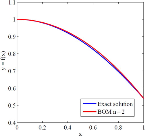
Comparison between the curves of exact solutions and the Bernstein operational matrix (BOM) solutions in case of $n=2$ is shown in Fig. 1. From this figure, it can be noted that the results of the present technique are an excellent agreement with the exact solution, they are more applicable and efficient for solving singular boundary value problem.

Example 4.2

Next we consider the following singular BVP [34] as(23) $-y^{″}\left(x\right)-\frac{2}{x}{y}^{\prime }\left(x\right)+\left(1-x^2\right)y\left(x\right)=x^4-2x^2+7$(23) (24) $\text{with}\text{boundary}\text{conditions}y\left(0\right)=1,y\left(1\right)=0.$(24)

Fig. 1 Comparison between exact and BOM solutions with $n=2$ for Example 4.1.

Eq. (23)(23) $-y^{″}\left(x\right)-\frac{2}{x}{y}^{\prime }\left(x\right)+\left(1-x^2\right)y\left(x\right)=x^4-2x^2+7$(23) has the exact solution of the boundary value problem and it is$y\left(x\right)=1-x^2$. As described in sections 2 and 3, Bernstein operational matrix technique leads to the system of algebraic equations, by solving them, the unknown coefficients of the vector $C$ calculated by using the following values$c_0=1,c_1=1,c_2=0.$

Thus, $y\left(x\right)-1-x^2$ is the exact solution of the given in Example 4.2

It is understandable that in Example 4.2, the proposed algorithm is speedily converged in to the true solution results. For a small value of $n=2$, the exact solution is reached. This proves the efficiency of the proposed BOM method.

The results obtained by BOM for $n=2$ are compared with the exact solution, and B-Spline results given in Ref. [3] are listed in Table 2. The absolute errors among exact, BOM and B-Spline methods are calculated. E₁ indicates the absolute errors between exact and BOM, whereas E₂ indicates the absolute errors between exact and B-Spline methods. Table 2 shows that the proposed method has high accuracy and has better results than the B-Spline method for all points of x. It is also clear that the proposed algorithm attains the exact solution by using very few calculations.

Example 4.3

Consider the Bessel's equation of order zero [35](25) $y^{″}\left(x\right)+\frac{1}{x}{y}^{\prime }\left(x\right)+y\left(x\right)=0$(25) with boundary conditions(26) $y^{\prime }\left(0\right)=0,y\left(1\right)=1$(26)

Table 2 Errors of the present method compared with B-Spline results for the Example 4.2.

x	Exact	BOM $n=2$ (E1)	B-Spline (E2)	Error by E1	Error by E2
0	1.0000	1.0000	0.9990	0	0.001
0.1	0.9900	0.9900	0.9899	0	1E-04
0.2	0.9600	0.9600	0.9599	0	1E-04
0.3	0.9100	0.9100	0.9099	0	1E-04
0.4	0.8400	0.8400	0.8399	0	1E-04
0.5	0.7500	0.7500	0.7499	0	1E-04
0.6	0.6400	0.6400	0.6399	0	1E-04
0.7	0.5100	0.5100	0.5099	0	1E-04
0.8	0.3600	0.3600	0.3599	0	1E-04
0.9	0.1900	0.1900	0.1900	0	0
1	0	0	0	0	0

The exact solution is $y\left(x\right)=\frac{J_0\left(x\right)}{J_0\left(1\right)}$.

By applying the method described in the sections 2 and 3 with $n=3$,

Eq. (25)(25) $y^{″}\left(x\right)+\frac{1}{x}{y}^{\prime }\left(x\right)+y\left(x\right)=0$(25) converted to the following equation:(27) $\left(\frac{13}{8}\right)c_0+\left(-\frac{33}{8}\right)c_1+\left(-\frac{9}{8}\right)c_2+\left(\frac{37}{8}\right)c_3=0.$(27)

Applying Eq. (15)(15) $\begin{array}{l}y\left(0\right)=C^{T}B\left(0\right)=a_1\text{},y\left(1\right)=C^{T}B\left(1\right)=b\left(\text{or}\right)\\ y^{\prime }\left(0\right)=C^{T}DB\left(0\right)=a_2\text{},y\left(1\right)=C^{T}B\left(1\right)=b\end{array}$(15) in the boundary conditions (26), we obtain(28) $-3c_0+3c_1=0$(28) (29) $c_3=1.$(29)

Solving the Eqs. (27)–(29), we get$c_0=1.3167,c_1=1.3167,c_2=1.1850,c_3=1.$

Consequently, we obtain$\begin{array}{c}y\left(x\right)=\left(1.3167,1.3167,1.1850,1\right)\left(\begin{array}{l}{\left(1-x\right)}^3\hfill \\ 3x{\left(1-x\right)}^2\hfill \\ 3x^2\left(1-x\right)\hfill \\ x^3\hfill \end{array}\right)\\ =\left(0.0784\right)x^3-\left(0.3951\right)x^2+1.3161\end{array}$

The numerical results are presented in the Table 3.

Table 3 Computed values and comparison to the exact solutions for the Example 4.3.

x	Exact	BOM $n=3$	Absolute error
0.1	1.3036	1.3128	0.0092
0.2	1.2939	1.3015	0.0076
0.3	1.2777	1.2833	0.0056
0.4	1.2552	1.2585	0.0033
0.5	1.2265	1.2277	0.0012
0.6	1.1919	1.1914	0.0005
0.7	1.1516	1.1500	0.0016
0.8	1.1060	1.1040	0.0020
0.9	1.0554	1.0538	0.0016
1	1	1	0

The proposed algorithm is applied to the well known Bessel's equation of order zero. The exact solution and BOM with $n=3$ solution are displayed in Table 3. The maximum absolute errors between BOM and exact solution for various choices of x are also shown in Table 3. It is clearly noted that the errors are very close to zero. This proves the efficiency of the proposed algorithm.

Example 4.4

Next we consider the following singular boundary value problem [35](30) $y^{″}\left(x\right)+\frac{2}{x}{y}^{\prime }\left(x\right)-4y\left(x\right)=-2$(30) (31) $\text{subject}\text{to}\text{the}\text{conditions}{y}^{\prime }\left(0\right)=0,y\left(1\right)=5.5$(31)

which has the exact solution of the boundary value problem $y\left(x\right)=\frac{1}{2}+\frac{5\sinh 2x}{x\sinh 2}$

This problem is solved by applying the method described in Sections 2 and 3.

Applying Bernstein operational matrices of derivatives with $n=3$ in Eq. (30)(30) $y^{″}\left(x\right)+\frac{2}{x}{y}^{\prime }\left(x\right)-4y\left(x\right)=-2$(30) and using the boundary conditions, the unknown coefficient values$\begin{array}{l}{c}_0=3.3,c_1=3.3,c_2=3.746\text{and}\\ c_4=5.5\text{are}\text{obtained}.\end{array}$(32) $\text{Then}\text{we}\text{get}y\left(x\right)=\left(0.86\right)x^3+\left(1.34\right)x^2+3.3.$(32)

The numerical results are presented in the Table 4.

Table 4 Computed values and comparison to the exact solutions for the Example 4.4.

x	Exact	BOM $n=3$	Absolute Error
0.1	3.2756	3.3143	0.0387
0.2	3.3313	3.605	0.0292
0.3	3.4256	3.4438	0.0182
0.4	3.5608	3.5694	0.0086
0.5	3.7402	3.7425	0.0023
0.6	3.9682	3.9682	0
0.7	4.2503	4.2516	0.0013
0.8	4.5937	4.5979	0.0042
0.9	5.0067	5.0123	0.0056
1	5.5000	5.5000	0

Maximum absolute errors for this problem have been displayed for $n=3$ in Table 4, which shows the accuracy of proposed method. From the exhibited results for this example in 4.4 show the advantage of this method.

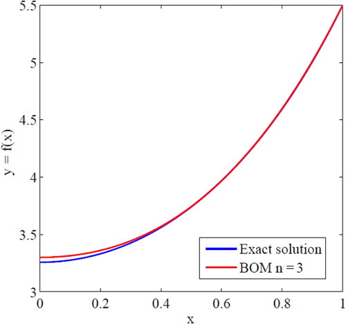
Fig. 2 illustrates a comparison between the curves of exact solutions and the approximate solutions. It can be concluded from Fig. 2 that the Bernstein operational matrix method solutions converge rapidly to the exact solution.

Example 4.5

Now, the general Lane-Emden type differential equation discussed by Rafiq et al. [36] is considered(33) $y^{″}+\frac{2}{x}{y}^{\prime }+x^r{y}^n=00\le x\le 1$(33) with boundary conditions(34) $y\left(0\right)=1,y^{\prime }\left(0=0\right).$(34)

Fig. 2 Comparison between exact and BOM solutions with $n=3$ for Example 4.4.

For the case $r=n=0$, Eq. (33)(33) $y^{″}+\frac{2}{x}{y}^{\prime }+x^r{y}^n=00\le x\le 1$(33) has the exact solution of the boundary value problem and it is $y\left(x\right)=1-\frac{x^2}{6}$.

As done before, the Lane-Emden type differential equation is solved. Applying the boundary conditions of Eq. (34)(34) $y\left(0\right)=1,y^{\prime }\left(0=0\right).$(34) in Eq. (33)(33) $y^{″}+\frac{2}{x}{y}^{\prime }+x^r{y}^n=00\le x\le 1$(33) and by following the same procedure given in Example 4.1 for the case corresponds to $n=2$.

Thus, Eq. (33)(33) $y^{″}+\frac{2}{x}{y}^{\prime }+x^r{y}^n=00\le x\le 1$(33) and Eq. (34)(34) $y\left(0\right)=1,y^{\prime }\left(0=0\right).$(34) are transformed into a system of algebraic equations. Solving the system of algebraic equations,

$c_0=1,c_1=1,c_2=\frac{5}{6}$ are obtained.

Then, $y\left(x\right)=\left(1,1,\frac{5}{6}\right)\left(\begin{array}{l}\left(1-x^2\right)\hfill \\ 2x\left(1-x\right)\hfill \\ x^2\hfill \end{array}\right)=1-\frac{x^2}{6}$ is the exact solution.

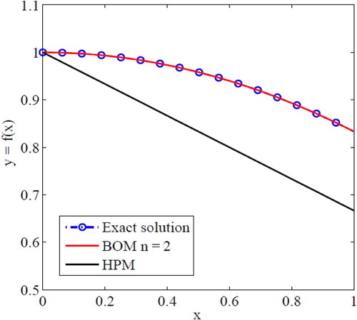
The exact solution of y(x), the approximate solutions of BOM and Homotopy Perturbation Method (HPM) are plotted in Fig. 3, Comparison between the solution obtained by using the proposed algorithm, HPM used by Rafiq et al. [36] and the exact solution are exhibited. It is observed from Fig. 3 that the present solution converges rapidly to the exact solution for small size of operational matrix and it is more accurate than the solution in Rafiq et al. [36]. The efficiency and power of the proposed algorithm are proved.

Example 4.6

Finally, consider the following initial value problem(35) $y^{″}\left(x\right)+\frac{1}{x}{y}^{\prime }\left(x\right)={\left(\frac{8}{8-x^2}\right)}^2$(35) with boundary conditions(36) $y^{\prime }\left(0\right)=0,y\left(1\right)=0$(36) which has the exact solution $2\log \left(\frac{7}{8-x^2}\right)$.

Fig. 3 Comparison between the BOM, HPM, and exact solutions of Example 4.5.

We solve problem Eq. (35)(35) $y^{″}\left(x\right)+\frac{1}{x}{y}^{\prime }\left(x\right)={\left(\frac{8}{8-x^2}\right)}^2$(35) by applying the method described in Sections 2 and 3, using Bernstein operational matrices of derivatives with $n=2$ we have$\begin{array}{l}{c}_0=-0.2663,c_1=-0.2663,c_2=0\text{and}\text{get}\\ y\left(x\right)=\left(0.2663\right)x^2-\left(0.2663\right).\end{array}$

Results in Table 5 show the comparison between the exact solutions and the BOM solutions for various values of x and $n=2$. The absolute errors are also given in Table 5. As seen from the table, it is evident that the overall errors are near to zero. This shows that the proposed approach is not only more accurate but also more simple and direct.

Table 5 Computed values and comparison to the exact solutions for the Example 4.6.

x	Exact	BOM $n=2$	Absolute error
0.1	–0.2646	–0.2636	0.0010
0.2	–0.257	–0.2556	0.0014
0.3	–0.2444	–0.2423	0.0021
0.4	–0.2267	–0.2237	0.0030
0.5	–0.2036	–0.1997	0.0039
0.6	–0.175	–0.1704	0.0046
0.7	–0.1407	–0.1358	0.0049
0.8	–0.1003	–0.0959	0.0044
0.9	–0.0536	–0.0506	0.0030
1	0	0	0

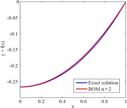
The curves of exact solutions and approximate solutions obtained by the proposed method for $n=2$ are shown in Fig. 4. In the figure, the exact and approximate solutions completely coincide. It is clear from this figure that the proposed solutions converge rapidly to the exact solution.

Fig. 4 Comparison between the results obtained from BOM and exact solution of Example 6.

5 Conclusion

In this work, a new spectral method is constructed for a numerical solution of the singular boundary value problems. Based on the Bernstein polynomials, the operational matrix derivatives are used together with the properties of Bernstein polynomials to reduce the given singular boundary value problems to a system of algebraic equations and it simplifies the problem. The main advantage of the proposed algorithm is adding few terms of the Bernstein polynomials, and a good approximation of the exact solution of the problem is achieved. The accuracy of the proposed BOM method has been demonstrated by solving widely applicable singular boundary value test problems.

Moreover, the proposed technique provides a reliable method which requires less work compared to the traditional techniques such as B-spline and standard HPM. The approach has been tested on some existing problems from the literature. From the comparison of the results made with some exact solutions, it can be concluded that the proposed approach is effective and viable to broad range of nonlinear singular boundary value problems. The results show that BOM method values match very effectively with the exact solution with very few calculations. By comparing the results with other existing methods, it has been proved that the proposed method provides more realistic solutions that convey very rapid convergence toward the exact solution.

Acknowledgment

The authors would like to thank the referee for his valuable comments and suggestions which improved the manuscript in its present form.