Deflection prediction of a cantilever beam subjected to static co-planar loading by analytical methods

Peer review under responsibility of Housing and Building National Research Center.

Abstract

In this paper, deflection prediction of a cantilever beam subjected to static co-planar loading is investigated using the Differential Transformation Method (DTM) and the Homotopy Perturbation Method (HPM). An axial compressive force, F_A, and a transverse force, Q_A, are applied to the beam. It is considered that these forces are follower forces, i.e., they will rotate with the end section of the beam during the deformation, and they will remain tangential and perpendicular at all times, respectively. Comparison between DTM and HPM through numerical results demonstrates that DTM can be an exact and highly efficient procedure for solving these kind of problems. Also the influence of the effect of some parameters appeared in mathematical formulations such as area moment of inertia (I), Young’s modulus (E), transverse force (Q_A) and compressive force (F_A) on slope variation are investigated in the present study. The results show that slope parameter as well as compressive force increases. By increasing the Q_A, slope parameter is increased significantly. By increasing the E, due to stiffness of the material, slope variation is decreased. It is evident that when the size of the beam section increases, the area moment of inertia (I) will be increased and so the slope variation will be decreased.

Keywords:

• Homotopy Perturbation Method
• Differential Transformation Method
• Slope parameter
• Co-planar loading
• Young’s modulus

Nomenclature
E	=	Young’s modulus
H	=	DTM transformed of η(s)
I	=	area moment of inertia
L	=	un-deformed length
FA	=	compressive force
QA	=	transverse force
s	=	arc length parameter
x	=	Cartesian coordinate – beam length direction
xA	=	x at beam end
y	=	Cartesian coordinate – beam thickness direction
yA	=	y at beam end
η	=	slope parameter
θ	=	slope of normal to beam cross section relative to x axis
θA	=	normal slope at the end section

Introduction

Most scientific problems in solid mechanics are inherently nonlinear by nature, and, except for a limited number of cases, most of them do not have analytical solutions. Accordingly, the nonlinear equations are usually solved using other methods including numerical techniques or by using analytical methods such as Homotopy Perturbation Methods. Therefore, obtaining analytical limit state functions or using analytical techniques to obtain reliability index for nonlinear problems is almost impossible. Analytical methods which recently are widely used are one of the simple and reliable methods for the solving system of coupled nonlinear differential equations. Following this two applicable analytical methods named the Homotopy Perturbation Method (HPM) and the Differential Transformation Method (DTM) are introduced.

HPM is an effective and convenient method for both linear and nonlinear equations. This method does not depend on a small parameter. This method was applied for many nonlinear problems some of which are introduced in [1–^[2][3]4]. Roozi et al. [5] used HPM to solve nonlinear parabolic–hyperbolic partial differential equations and presented examples of one-dimension and two-dimensions to show the ability of the method for such equations. Ganji and Sadighi [6] applied HPM for solving nonlinear heat transfer and porous media equations also they introduced HPM to obtain the exact solutions of linear and nonlinear Schrödinger equations [7]. Sadighi and Ganji [8] obtained the exact solutions of the Laplace equation with Dirichlet and Neumann boundary conditions using HPM. Ziabakhsh and Domairry [9] have studied the natural convection of a non-Newtonian fluid between two infinite parallel vertical flat plates and the effects of the non-Newtonian nature of fluid on the heat transfer by HPM. Ganji et al. [10] considered two known nonlinear systems which are different in phenomena but same in practice. The resulted nonlinear differential equation was separately solved by using the HPM and compared with numerical solution. Also Khavaji et al. [11] applied HPM for finding the large deflections subject in compliant mechanisms.

The differential transform method (DTM) is based on the Taylor expansion. It constructs an analytical solution in the form of a polynomial. It is different from the traditional high order Taylor series method, which requires symbolic computation of the necessary derivatives of the data functions. This method was first applied in the engineering domain by Zhou [12] and its abilities have attracted many authors to use this method for solving nonlinear equations. Following this some of these works are introduced. Ghafoori et al. [13] solved a nonlinear oscillation equation using DTM and as an important result, they revealed that the DTM results are more accurate in comparison with those obtained by HPM and VIM. Ravi Kanth and Aruna [14] solved linear and nonlinear Klein–Gordon equations by DTM. Biazar and Eslami [15] considered DTM to solve the quadratic Riccati differential equation. Their results derived by differential transform method were compared with the results of the homotopy analysis method and the Adomian decomposition method and it was shown that DTM used for quadratic Riccati differential equation was more effective and promising than the homotopy analysis method and the Adomain decomposition method. Gokdogan et al. [16] acquired an approximate analytical solution of the chaotic Genesio system by the modified differential transform method. Ayaz [17] has studied the two-dimensional differential transform method of solution of the initial value problem for partial differential equations (PDEs). Gorji et al. [18] used DTM for illustrating the efficiency of air-heating solar collectors.

In this paper, HPM and DTM are applied for the first time to analytically obtain the slope variation of a beam subjected to co-planer loading. As an important result, it is depicted that the DTM results are more accurate in comparison with those obtained by HPM. After this verification, the effects of some physical applicable parameters are investigated to show the efficiency of DTM for these type of problems.

Mathematical formulation

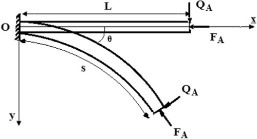
A cantilever beam OA is subjected to co-planar loading consisting of an axial compressive force F_A and of a transverse force Q_A (Fig. 1). F_A and Q_A are follower forces, i.e., they will rotate with the end section A of the beam during the deformation, and they will at all times remain tangential and perpendicular, respectively, to the deformed beam axis. It is assumed that the effect of the material nonlinearity is negligible in the mathematical derivation. Therefore, at any point of coordinates x(s), y(s) the external moment M is expressed as [19]:(1) $M=(F_A\cos {\theta }_A+Q_A\sin {\theta }_A)(y_A·y)+(F_A\sin {\theta }_A+Q_A\cos {\theta }_A)(x_A·y)$(1) where x, y are the longitudinal and transverse coordinates, respectively, q is the slope of the normal to the beam cross section, and x_A, y_A and θ_A denote the coordinates and the normal slope at the end section. The classical Euler–Bernoulli hypothesis assumes that the bending moment M at any point of the beam is proportional to the corresponding curvature i.e.(2) $M=\mathit{EI}{\theta }^{\prime }$(2) where E is Young’s modulus, and I is the area moment of inertia of the beam cross section about the x axis. By using the following relations:(3) $\frac{\mathit{dx}}{\mathit{ds}}=\cos \theta \text{,}\frac{\mathit{dy}}{\mathit{ds}}=\sin \theta$(3) and based on the trigonometric relations and by substituting Eqs. (2(2) $M=\mathit{EI}{\theta }^{\prime }$(2) and3(3) $\frac{\mathit{dx}}{\mathit{ds}}=\cos \theta \text{,}\frac{\mathit{dy}}{\mathit{ds}}=\sin \theta$(3) ) into Eq. (1(1) $M=(F_A\cos {\theta }_A+Q_A\sin {\theta }_A)(y_A·y)+(F_A\sin {\theta }_A+Q_A\cos {\theta }_A)(x_A·y)$(1) ), the nonlinear differential equation governing the problem is obtained as follows:(4) $\frac{{\partial }^2\eta }{\partial s^2}+\frac{F_A}{\mathit{EI}}\sin (\eta (s))+\frac{Q_A}{\mathit{EI}}\cos (\eta (s))=0$(4)

Fig. 1 The geometry of a cantilever beam subjected to non-conservative external loading (follower forces).

The boundary conditions associated with the above equation are,(5) $\eta (0)=0\text{,}{\eta }^{\prime }(L)=0$(5) where,(6) $\eta =\theta -{\theta }_A$(6)

Using only the two terms of a Taylor’s series expansion for cos(η(s)) and sin(η(s)), and substituting in Eq. (4(4) $\frac{{\partial }^2\eta }{\partial s^2}+\frac{F_A}{\mathit{EI}}\sin (\eta (s))+\frac{Q_A}{\mathit{EI}}\cos (\eta (s))=0$(4) ) yields:(7) $\frac{{\partial }^2\eta }{\partial s^2}+\frac{F_A}{\mathit{EI}}\left(\eta (s)-\frac{1}{6}{\eta }^3(s)\right)+\frac{Q_A}{\mathit{EI}}\left(1-\frac{1}{2}{\eta }^2(s)\right)=0$(7)

Analytical methods and applications

Differential Transformation Method (DTM)

In this section the fundamental basic of the Differential Transformation Method is introduced. For understanding method’s concept, suppose that x(t) is an analytic function in domain D, and t = t_i represents any point in the domain. The function x(t) is then represented by one power series whose center is located at t_i. The Taylor series expansion function of x(t) is in the form of:(8) $x(t)={\displaystyle \sum _{k=0}^{\infty }}\frac{{\left(t-t_i\right)}^k}{k!}{\left[\frac{d^{k}x(t)}{{\mathit{dt}}^k}\right]}_{t=t_i}\forall t\in D$(8)

The Maclaurin series of x(t) can be obtained by taking t_i = 0 in Eq. (8(8) $x(t)={\displaystyle \sum _{k=0}^{\infty }}\frac{{\left(t-t_i\right)}^k}{k!}{\left[\frac{d^{k}x(t)}{{\mathit{dt}}^k}\right]}_{t=t_i}\forall t\in D$(8) ) expressed as:(9) $x(t)={\displaystyle \sum _{k=0}^{\infty }}\frac{t^k}{k!}{\left[\frac{d^{k}x(t)}{{\mathit{dt}}^k}\right]}_{t=0}\forall t\in D$(9)

As explained in [12] the differential transformation of the function x(t) is defined as follows:(10) $X(k)={\displaystyle \sum _{k=0}^{\infty }}\frac{H^k}{k!}{\left[\frac{d^{k}x(t)}{{\mathit{dt}}^k}\right]}_{t=0}$(10) where X(k) represents the transformed function and x(t) is the original function. The differential spectrum of X(k) is confined within the interval $t\in [0\text{,}H]$, where H is a constant value. The differential inverse transform of X(k) is defined as follows:(11) $x(t)={\displaystyle \sum _{k=0}^{\infty }}{\left(\frac{t}{H}\right)}^{k}X(k)$(11)

It is clear that the concept of differential transformation is based upon the Taylor series expansion. The values of function X(k) at values of argument k are referred to as discrete, i.e. X(0) is known as the zero discrete, X(1) as the first discrete, etc. The more discrete available, the more precise it is possible to restore the unknown function. The function x(t) consists of the T-function X(k), and its value is given by the sum of the T-function with (t/H)k as its coefficient. In real applications, at the right choice of constant H, the larger the values of argument k the discrete of the spectrum reduces rapidly. The function x(t) is expressed by a finite series and Eq. (11(11) $x(t)={\displaystyle \sum _{k=0}^{\infty }}{\left(\frac{t}{H}\right)}^{k}X(k)$(11) ) can be written as:(12) $x(t)={\displaystyle \sum _{k=0}^{\infty }}{\left(\frac{t}{H}\right)}^{k}X(k)$(12)

Some important mathematical operations performed by differential transform method are listed in Table 1.

Table 1 Some fundamental operations of the differential transform method.

Origin function	Transformed function
x(t) = αf(x) ± βg(t)	X(k) = αF(k) ± βG(k)
$x(t)=\frac{d^{m}f(t)}{{\mathit{dt}}^m}$	$X(k)=\frac{(k+m)!F(k+m)}{k!}$
x(t) = f(t) g(t)	$X(k)=\sum _{l=0}^{k}F(l)G(k-l)$
x(t) = t^m	$X(k)=\delta (k-m)=\left\{\begin{array}{c}\hfill 1\text{,if}k=m\text{,}\hfill \\ \hfill 0\text{,if}k\ne m\text{.}\hfill \end{array}\right.$
x(t) = exp(t)	$X(k)=\frac{1}{k!}$
x(t) = sin(ωt + α)	$X(k)=\frac{{\omega }^k}{k!}\sin \left(\frac{k\pi }{2}+\alpha \right)$
x(t) = cos(ωt + α)	$X(k)=\frac{{\omega }^k}{k!}\cos \left(\frac{k\pi }{2}+\alpha \right)$

Application of DTM

Now Differential Transformation Method (DTM) is applied from Table 1 into Eq. (7(7) $\frac{{\partial }^2\eta }{\partial s^2}+\frac{F_A}{\mathit{EI}}\left(\eta (s)-\frac{1}{6}{\eta }^3(s)\right)+\frac{Q_A}{\mathit{EI}}\left(1-\frac{1}{2}{\eta }^2(s)\right)=0$(7) ) for find η(s). So:(13) $(k+1)(k+2)H(k+2)+\frac{F_A}{\mathit{EI}}H(k)-\left(\frac{F_A}{\mathit{EI}}\right)\left(\frac{1}{6}\right){\displaystyle \sum _{k1=0}^k}{\displaystyle \sum _{l=0}^{k1}}H(l)H(k1-l)H(k-k1)+\frac{Q_A}{\mathit{EI}}\delta [k]-\left(\frac{Q_A}{\mathit{EI}}\right)\left(\frac{1}{2}\right){\displaystyle \sum _{l=0}^k}H(l)H(k-l)=0$(13) where,(14) $\delta [k]=\left\{\begin{array}{cc}1\hfill & \text{if}k=0\hfill \\ 0\hfill & \text{if}k\ne 0\hfill \end{array}\right.$(14)

Similarly, the transformed form of boundary conditions (Eq. (5(5) $\eta (0)=0\text{,}{\eta }^{\prime }(L)=0$(5) )) can be written as:(15) $H(0)=0\text{,}H(1)=a$(15) in which the boundary condition of this case is the same as in the previous case. By solving Eq. (13(13) $(k+1)(k+2)H(k+2)+\frac{F_A}{\mathit{EI}}H(k)-\left(\frac{F_A}{\mathit{EI}}\right)\left(\frac{1}{6}\right){\displaystyle \sum _{k1=0}^k}{\displaystyle \sum _{l=0}^{k1}}H(l)H(k1-l)H(k-k1)+\frac{Q_A}{\mathit{EI}}\delta [k]-\left(\frac{Q_A}{\mathit{EI}}\right)\left(\frac{1}{2}\right){\displaystyle \sum _{l=0}^k}H(l)H(k-l)=0$(13) ) and using boundary conditions Eq. (15(15) $H(0)=0\text{,}H(1)=a$(15) ), the DTM terms for this case for F_A = 300 KN, Q_A = 350 KN, E = 40 GPa and I = 1.6 × 10⁻⁵ m⁴ can be:(16) $\begin{array}{cc}\hfill & H(2)=-0.2734375000\hfill \\ \hfill & H(3)=-0.7812500000a\hfill \\ \hfill & H(4)=0.1068115234+0.02278645833a^2\hfill \\ \hfill & H(5)=-0.005645751950a+0.003906250000a^3\hfill \end{array}$(16) etc.

Now by applying Eq. (11(11) $x(t)={\displaystyle \sum _{k=0}^{\infty }}{\left(\frac{t}{H}\right)}^{k}X(k)$(11) ) in to Eq. (16(16) $\begin{array}{cc}\hfill & H(2)=-0.2734375000\hfill \\ \hfill & H(3)=-0.7812500000a\hfill \\ \hfill & H(4)=0.1068115234+0.02278645833a^2\hfill \\ \hfill & H(5)=-0.005645751950a+0.003906250000a^3\hfill \end{array}$(16) ), and using Eq. (15(15) $H(0)=0\text{,}H(1)=a$(15) ) the constant parameter “a” will be obtained so the slope parameter equation will be estimated:(17) $\eta (s)=a·s-0.2734375000s^2-0.07812500000a·s^3+(0.01068115234+0.02278645833a^2)s^4+(-0.005645751950a+0.003906250000a^3)s^5+(0.0005145867667-0.003916422527a^2)s^6+(0.0008974756514a-0.0001828632660a^3)s^7+(-0.00006135087461+0.0001701215902a^2+0.0001335144043a^4)s^8$(17)

By using boundary condition in s = 1, the ‘a’ parameter will be determined as:(18) $a=0.6310718570$(18) and by substituting it into Eq. (17(17) $\eta (s)=a·s-0.2734375000s^2-0.07812500000a·s^3+(0.01068115234+0.02278645833a^2)s^4+(-0.005645751950a+0.003906250000a^3)s^5+(0.0005145867667-0.003916422527a^2)s^6+(0.0008974756514a-0.0001828632660a^3)s^7+(-0.00006135087461+0.0001701215902a^2+0.0001335144043a^4)s^8$(17) ), η(s) will be found as:(19) $\eta (s)=0.6310718570s-0.2734375000s^2-0.04930248883s^3+0.01975589785s^4-0.002581135196s^5-0.001045135118s^6+0.0005204134364s^7+0.00002757630897s^8$(19)

Homotopy Perturbation Method (HPM)

In this section, Homotopy Perturbation Method is applied to the discussed problem. To illustrate the basic ideas of this method, the following nonlinear differential equation is considered:(20) $A(u)-f(r)=0\text{,}r\in \mathrm{\Omega }$(20)

With boundary conditions of:(21) $B\left(u\text{,}\frac{\partial u}{\partial n}\right)=0\text{,}r\in \mathrm{\Gamma }$(21) where A(u) is defined as follows:(22) $A(u)=L(u)+N(u)$(22)

By the homotopy technique, we construct a homotopy as v(r,p): Ω × [0,1]→ which satisfies:(23) $H(\nu \text{,}p)=(1-p)[L(\nu )-L(u_0)]+p[A(\nu )-f(r)]=0P\in [0\text{,}1]\text{,}r\in \mathrm{\Omega }$(23) or:(24) $H(\nu \text{,}p)=L(\nu )-L(u_0)+\mathit{pL}(u_0)+p[N(\nu )-f(r)]=0$(24)

Obviously, using Eq. (23(23) $H(\nu \text{,}p)=(1-p)[L(\nu )-L(u_0)]+p[A(\nu )-f(r)]=0P\in [0\text{,}1]\text{,}r\in \mathrm{\Omega }$(23) ) we have:(25) $H(\nu \text{,}0)=L(\nu )-L(u_0)=0\text{,}H(\nu \text{,}1)=A(\nu )-f(r)=0\text{.}$(25) where $p\in [0\text{,}1]$ is an embedding parameter and u₀ is the first approximation that satisfies the boundary condition. The process of changes in p from 0 to unity is that of ν(r,p) changing from u₀ to u(r). We consider ν, as the following:(26) $\nu ={\nu }_0+p{\nu }_1+p^2{\nu }_2+p^3{\nu }_3+\dots$(26) and the best approximation for the solution is:(27) $u={\displaystyle \underset{p\to 1}{\lim }}=\nu ={\nu }_0+{\nu }_1+{\nu }_2+\dots$(27)

Application of HPM

According to the Homotopy Perturbation Method (HPM), we construct a homotopy. Suppose the solution of Eq. (7(7) $\frac{{\partial }^2\eta }{\partial s^2}+\frac{F_A}{\mathit{EI}}\left(\eta (s)-\frac{1}{6}{\eta }^3(s)\right)+\frac{Q_A}{\mathit{EI}}\left(1-\frac{1}{2}{\eta }^2(s)\right)=0$(7) ) has the form:(28) $H(\eta \text{,}p)=(1-p)\left[\frac{{\partial }^2\eta }{\partial s^2}+\frac{F_A}{\mathit{EI}}(\eta (s))\right]+p\left[\frac{{\partial }^2\eta }{\partial s^2}+\frac{F_A}{\mathit{EI}}\left(\eta (s)-\frac{1}{6}{\eta }^3(s)\right)+\frac{Q_A}{\mathit{EI}}\left(1-\frac{1}{2}{\eta }^2(s)\right)\right]=0$(28)

It is considered that:(29) $\eta (s)={\eta }_0(s)+p{\eta }_1(s)+p^2{\eta }_2(s)+\dots ={\displaystyle \sum _{i=0}^n}{p}^i{\eta }_i(s)$(29)

By substituting η from Eq. (29(29) $\eta (s)={\eta }_0(s)+p{\eta }_1(s)+p^2{\eta }_2(s)+\dots ={\displaystyle \sum _{i=0}^n}{p}^i{\eta }_i(s)$(29) ) into Eq. (28(28) $H(\eta \text{,}p)=(1-p)\left[\frac{{\partial }^2\eta }{\partial s^2}+\frac{F_A}{\mathit{EI}}(\eta (s))\right]+p\left[\frac{{\partial }^2\eta }{\partial s^2}+\frac{F_A}{\mathit{EI}}\left(\eta (s)-\frac{1}{6}{\eta }^3(s)\right)+\frac{Q_A}{\mathit{EI}}\left(1-\frac{1}{2}{\eta }^2(s)\right)\right]=0$(28) ) and some simplification and rearranging based on powers of p-terms, we have:(30) $\begin{array}{c}\hfill p^0:\frac{F_A{\eta }_0(s)}{\mathit{EI}}+\frac{d^2{\eta }_0(s)}{{\mathit{ds}}^2}=0\hfill \\ \hfill {\eta }_0(0)=0\text{,}{\eta }_0^{\prime }(L)=0\hfill \end{array}$(30) (31) $\begin{array}{c}\hfill p^1:\frac{F_A{\eta }_1(s)}{\mathit{EI}}+\frac{Q_A}{\mathit{EI}}+\frac{d^2{\eta }_1(s)}{{\mathit{ds}}^2}-\frac{1}{2}\frac{Q_A{\eta }_0^2(s)}{\mathit{EI}}-\frac{1}{6}\frac{F_A{\eta }_0^3(s)}{\mathit{EI}}=0\hfill \\ \hfill {\eta }_1(0)=0\text{,}{\eta }_1^{\prime }(L)=0\hfill \end{array}$(31) (32) $\begin{array}{c}\hfill p^2:\frac{F_A{\eta }_2(s)}{\mathit{EI}}+\frac{d^2{\eta }_2(s)}{{\mathit{ds}}^2}-\frac{Q_A{\eta }_0(s){\eta }_1(s)}{\mathit{EI}}-\frac{1}{2}\frac{F_A{\eta }_0^2(s){\eta }_1(s)}{\mathit{EI}}=0\hfill \\ \hfill {\eta }_2(0)=0\text{,}{\eta }_2^{\prime }(L)=0\hfill \end{array}$(32) (33) $\begin{array}{c}\hfill p^3:\frac{F_A{\eta }_3(s)}{\mathit{EI}}+\frac{d^2{\eta }_3(s)}{{\mathit{ds}}^2}-\frac{1}{2}\frac{F_A{\eta }_0(s){\eta }_1^2(s)}{\mathit{EI}}-\frac{1}{2}\frac{Q_A{\eta }_1^2(s)}{\mathit{EI}}\hfill \\ \hfill -\frac{Q_A{\eta }_0(s){\eta }_2(s)}{\mathit{EI}}-\frac{1}{2}\frac{F_A{\eta }_0^2(s){\eta }_2(s)}{\mathit{EI}}=0\hfill \\ \hfill {\eta }_3(0)=0\text{,}{\eta }_3^{\prime }(L)=0\hfill \end{array}$(33)

Solving Eqs. (30(30) $\begin{array}{c}\hfill p^0:\frac{F_A{\eta }_0(s)}{\mathit{EI}}+\frac{d^2{\eta }_0(s)}{{\mathit{ds}}^2}=0\hfill \\ \hfill {\eta }_0(0)=0\text{,}{\eta }_0^{\prime }(L)=0\hfill \end{array}$(30) –⁽³¹⁾(31) $\begin{array}{c}\hfill p^1:\frac{F_A{\eta }_1(s)}{\mathit{EI}}+\frac{Q_A}{\mathit{EI}}+\frac{d^2{\eta }_1(s)}{{\mathit{ds}}^2}-\frac{1}{2}\frac{Q_A{\eta }_0^2(s)}{\mathit{EI}}-\frac{1}{6}\frac{F_A{\eta }_0^3(s)}{\mathit{EI}}=0\hfill \\ \hfill {\eta }_1(0)=0\text{,}{\eta }_1^{\prime }(L)=0\hfill \end{array}$(31) ⁽³²⁾(32) $\begin{array}{c}\hfill p^2:\frac{F_A{\eta }_2(s)}{\mathit{EI}}+\frac{d^2{\eta }_2(s)}{{\mathit{ds}}^2}-\frac{Q_A{\eta }_0(s){\eta }_1(s)}{\mathit{EI}}-\frac{1}{2}\frac{F_A{\eta }_0^2(s){\eta }_1(s)}{\mathit{EI}}=0\hfill \\ \hfill {\eta }_2(0)=0\text{,}{\eta }_2^{\prime }(L)=0\hfill \end{array}$(32) 33(33) $\begin{array}{c}\hfill p^3:\frac{F_A{\eta }_3(s)}{\mathit{EI}}+\frac{d^2{\eta }_3(s)}{{\mathit{ds}}^2}-\frac{1}{2}\frac{F_A{\eta }_0(s){\eta }_1^2(s)}{\mathit{EI}}-\frac{1}{2}\frac{Q_A{\eta }_1^2(s)}{\mathit{EI}}\hfill \\ \hfill -\frac{Q_A{\eta }_0(s){\eta }_2(s)}{\mathit{EI}}-\frac{1}{2}\frac{F_A{\eta }_0^2(s){\eta }_2(s)}{\mathit{EI}}=0\hfill \\ \hfill {\eta }_3(0)=0\text{,}{\eta }_3^{\prime }(L)=0\hfill \end{array}$(33) ) with boundary conditions for L = 1, we have:(34) ${\eta }_0(s)=0$(34) (35) ${\eta }_1(s)=\frac{\sin \left(\frac{s\sqrt{F_A}}{\sqrt{E}\sqrt{I}}\right)\sin \left(\frac{\sqrt{F_A}}{\sqrt{E}\sqrt{I}}\right)Q_A}{\cos \left(\frac{\sqrt{F_A}}{\sqrt{E}\sqrt{I}}\right)F_A}+\frac{\cos \left(\frac{s\sqrt{F_A}}{\sqrt{E}\sqrt{I}}\right)Q_A}{F_A}-\frac{Q_A}{F_A}$(35) (36) ${\eta }_2(s)=0$(36) etc.

With include Eqs. (30(30) $\begin{array}{c}\hfill p^0:\frac{F_A{\eta }_0(s)}{\mathit{EI}}+\frac{d^2{\eta }_0(s)}{{\mathit{ds}}^2}=0\hfill \\ \hfill {\eta }_0(0)=0\text{,}{\eta }_0^{\prime }(L)=0\hfill \end{array}$(30) –33(33) $\begin{array}{c}\hfill p^3:\frac{F_A{\eta }_3(s)}{\mathit{EI}}+\frac{d^2{\eta }_3(s)}{{\mathit{ds}}^2}-\frac{1}{2}\frac{F_A{\eta }_0(s){\eta }_1^2(s)}{\mathit{EI}}-\frac{1}{2}\frac{Q_A{\eta }_1^2(s)}{\mathit{EI}}\hfill \\ \hfill -\frac{Q_A{\eta }_0(s){\eta }_2(s)}{\mathit{EI}}-\frac{1}{2}\frac{F_A{\eta }_0^2(s){\eta }_2(s)}{\mathit{EI}}=0\hfill \\ \hfill {\eta }_3(0)=0\text{,}{\eta }_3^{\prime }(L)=0\hfill \end{array}$(33) ) and Eqs. (34(34) ${\eta }_0(s)=0$(34) –36(36) ${\eta }_2(s)=0$(36) ) in Eq. (29(29) $\eta (s)={\eta }_0(s)+p{\eta }_1(s)+p^2{\eta }_2(s)+\dots ={\displaystyle \sum _{i=0}^n}{p}^i{\eta }_i(s)$(29) ) and insert F_A = 300 KN, Q_A = 350 KN, E = 40 GPa and I = 1.6 × 10⁻⁵ m⁴ solution is as follows:(37) $\eta (s)=(0.7060861184)\sin (0.6846531969s)-(0.1123593318)\cos (0.6846531969s)+(0.2888947394)-(0.2205266417)\cos (1.369306394s-1.369306394)-(0.3307899626)\cos (1.369306394+0.6846531969s)-(0.3307899626)\cos (0.6846531969s-1.369306394)-(0.4529528108)(s)(\sin (0.6846531969s-1.369306394))-(0.4529528108)(s)(\sin (0.6846531969s))$(37)

Fourth-order Runge–Kutta numerical method

It is obvious that the type of the current problem is the boundary value problem (BVP) and the appropriate method needs to be chosen. The available sub-methods in the Maple 15.0 are a combination of the base schemes; trapezoid or midpoint method. There are two major considerations when choosing a method for a problem. The trapezoid method is generally efficient for typical problems, but the midpoint method is also capable of handling harmless end-point singularities that the trapezoid method cannot. The midpoint method, also known as the fourth-order Runge–Kutta–Fehlberg method, improves the Euler method by adding a midpoint in the step which increases the accuracy by one order. Thus, the midpoint method is used as a suitable numerical technique in the present study [20].

Results and discussion

Deflection of a cantilever beam subjected to static co-planar loading by two analytical methods called HPM and DTM and the fourth order Runge–Kutta numerical method is investigated in the present study. For showing the efficiency of these analytical methods, Fig. 2 is presented. As seen in most cases of these figures, HPM and DTM have an excellent agreement with numerical solution but in some cases (for example when F_A = 100 KN, Q_A = 100 KN, E = 10⁹ Pa & I = 10⁻⁴ m⁴ see Fig. 2) the accuracy of the DTM is greater than HPM. Table 2 compared the results of the HPM and DTM with the numerical procedure and the Homotopy Analysis Method (HAM) which are presented by [19,21] when F_A = 300 KN, Q_A = 350 KN, E = 40 GPa and I = 1.6 × 10⁻⁵ m⁴. These data and calculated errors confirm that these two analytical methods are suitable and semi-exact for solving these kinds of problems. In the following step, effect of some parameters appeared in the mathematical formulation such as area moment of inertia (I), Young’s modulus (E), transverse force (Q_A) and compressive force (F_A) on slope variation are investigated. Selected values for showing the variation of these parameters are considered according to the mean value of stress limit state concluded from [19]. These mean values are presented in Table 3.

Fig. 2 Comparison of Slope parameter for HPM, DTM and Numerical solution when, (I) F_A = 400 KN, Q_A = 450 KN, E = 40 GPa & I = 7 × 10⁻⁵ m⁴. (II) F_A = 300 KN, Q_A = 350 KN, E = 40 GPa & I = 1.6 × 10⁻⁵ m⁴. (III) F_A = 100 KN, Q_A = 50 KN, E = 10⁹ Pa & I = 10⁻⁴ m⁴. (IV) F_A = 100 KN, Q_A = 100 KN, E = 10⁹ Pa & I = 10⁻⁴.

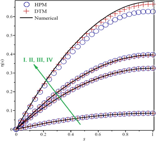
Table 2 Comparison between HPM, DTM and numerical solution for F_A = 300 KN, Q_A = 350 KN, E = 40 GPa and I = 1.6 × 10⁻⁵ m⁴.

s	η(s)Numerical	η(s)HAM [19,21]	η(s)HPM	η(s)DTM	(%) ErrorHPM	(%) ErrorDTM
0.1	0.06036251	0.06034326	0.06035369	0.06032545	0.00014625	0.00061397
0.2	0.11498708	0.11495123	0.11497007	0.11491317	0.00014793	0.00064274
0.3	0.16364459	0.16356398	0.16362082	0.16353411	0.00014527	0.00067508
0.4	0.20614594	0.20615968	0.20611719	0.20599929	0.00013944	0.00071139
0.5	0.24233792	0.24234267	0.24230515	0.24215566	0.00013523	0.00075207
0.6	0.27209923	0.27215896	0.27206024	0.27188220	0.00014331	0.00079763
0.7	0.29533656	0.29535986	0.29528238	0.29508623	0.00018348	0.00084760
0.8	0.31198116	0.31195631	0.31189042	0.31170062	0.00029085	0.00089921
0.9	0.32198607	0.32195632	0.32181657	0.32168184	0.00052643	0.00094486
1	0.32532409	0.32501035	0.32500059	0.32500948	0.00099440	0.00096706

Table 3 Mean values for parameters according to stress limit state presented in [19].

Parameter	Mean value
Shear force (QA)	350 (KN)
Normal force (FA)	300 (KN)
Young’s modulus (E)	40 (GPa)
Area moment of inertia (I)	2.6 E − 5 (m^4)

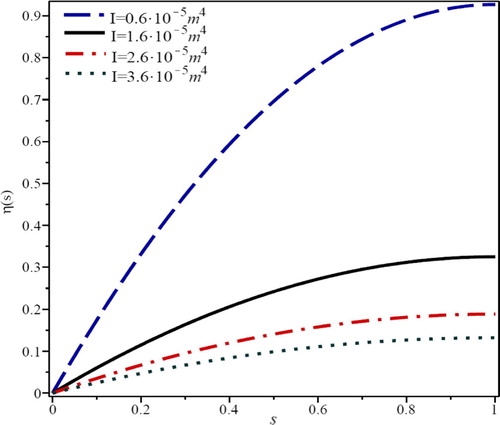
Effect of compressive force (F_A) on slope parameter, η(s), is presented in Fig. 3. As seen in this figure, slope parameter increases as well as compressive force increases. Variation of slope parameter based on transverse force (Q_A) is depicted in Fig. 4. By increasing the Q_A, slope parameter is increased significantly. From these two figures, it is evident that the effect of Q_A for increasing the slope parameter is more than F_A. It is due to their direction applied to the beam which as Fig. 1 shows, Q_A is a shear force and exerts more effects on the beam slope parameter. Fig. 5 shows the effect of Young’s modulus (E) on η(s). By increasing the E, due to stiffness of the material, slope variation is decreased. It is evident that when the size of the beam section increases, the area moment of inertia (I) will be increased, so the slope variation will be decreased. This fact is presented by Fig. 6.

Fig. 3 Effect of compressive force for Q_A = 350 KN, E = 40 GPa & I = 1.6 × 10⁻⁵ m⁴.

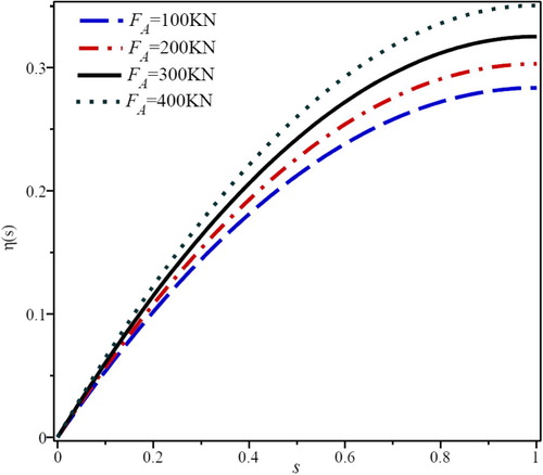
Fig. 4 Effect of transverse force for F_A = 300 KN, E = 40 GPa & I = 1.6 × 10⁻⁵ m⁴.

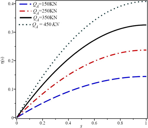
Fig. 5 Effect of Young’s modulus for F_A = 300 KN, Q_A = 350 KN & I = 1.6 × 10⁻⁵ m⁴.

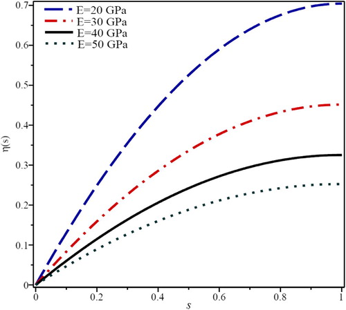
Fig. 6 Effect of area moment of inertia (I) for F_A = 300 KN, Q_A = 350 KN & E = 40 GPa.

Conclusion

In this paper, Differential Transformation Method (DTM) and Homotopy Perturbation Method (HPM) have been successfully applied to find the solution of the slope parameter of a cantilever beam subjected to co-planar loading consisting of an axial compressive force and a transverse force. Obtained solutions revealed that DTM and HPM can be simple, powerful and efficient techniques for finding analytical solutions of these kinds of physical problems with nonlinear differential equations. The results show that increasing the Young’s modulus and moment of inertia decreased the slope variations but increasing each of the transverse or compressive forces increased it.

Conflict of interest

The authors declare no conflict of interests.

Notes

Peer review under responsibility of Housing and Building National Research Center.