Long-term load forecasting for the Kingdom of Bahrain using Monte Carlo method

Abstract

The present study applies Monte Carlo method to electric power network of the Kingdom of Bahrain over a period of five years taking into consideration the maximum electrical loads. The basic variables of the Monte Carlo method are presented and discussed from the standard deviation and reserve points of view. The maximum loads and simulation results were compared on a weekly and yearly basis. A comparison of the minimum mean square error has been calculated and plotted. The results show similarity between the forecasted data and simulation results.

Keywords:

• Monte Carlo
• Mean square error
• Load

1 Introduction

Without the aid of simulation, a spreadsheet model will only reveal a single outcome. In the present study a number of values were needed to be generated (http://www.crystalball.com/monte-carlo-simulation.html). Hence we use the Monte Carlo simulation, which randomly generates values for uncertain variables over and over to simulate a model. The Kingdom of Bahrain’s electrical load over a number of years is taken into the consideration and the Monte Carlo method is implemented. The random behavior in problems of chance is similar to how Monte Carlo simulation selects variable values at random to simulate a model (http://www.crystalball.com/monte-carlo-simulation.html). A simulation calculates multiple scenarios of a model by repeatedly sampling values from the probability distributions for the uncertain variables and using those values for the cell (http://www.crystalball.com/monte-carlo-simulation.html). Applications of Monte Carlo techniques can be obtained in many fields, such as stochastic process simulation, complex mathematical calculations, medical statistics, reliability evaluation, and engineering system analysis.

Skeffington et al. tested four contrasting sites models for calculating critical loads for the deposition of acidity and nitrogen in forest and heath land ecosystem (Skeffington et al., 2007). Output distributions of various critical load parameters were calculated. The results were assessed by Monte Carlo methods. Overall, the analysis provided objective support for the continued use of critical loads in policy development.

Yi Ding et al. in their study discussed in reference (Ding et al., 2007) present a technique to evaluate reliability of a restructured power system with a bilateral market. The network has been implemented in the Monte Carlo simulation procedure to reduce the computational burden of the analysis. A new load shedding is proposed during generation inadequacy and network congestion to minimize the load curtailment.

In reference (Poulin et al., 2007), the authors discuss in their study that by considering the relationship between the electric power demand and time, the accuracy and relevance of energy solution analysis for a customer could be greatly improved. Through Monte Carlo simulations, the algorithm for generation of realistic synthetic load duration curve can be implemented. Some results for the assessment are presented in the study.

Researchers (Conti and Raiti, 2007) had presented solution of the load flow problem in distribution networks with photovoltaic (PV) distributed generation (DG). The proposed models have been incorporated in a radial distribution probabilistic load flow (PLF) program that has been developed using Monte Carlo techniques.

Ning Yang et al. in their paper (Yang et al., 2007) presented a novel method for reactive power planning based on chance constrained programming with uncertain factors taken into account. Using the Monte Carlo simulation method, the novel method is presented for solving the optimization problem.

In reference (Shin et al., 2007; Qader and Qamber, 2007), the authors suggest a probabilistic approach to calculate available transfer capability in the interconnected network. The evaluation of the transmission reliability margin and capacity benefit margin are evaluated by probabilistic load flow and Monte Carlo simulation. The proposed method is applied to a modified IEEE 72-bus three area system to calculate available transfer capability on two different time spans.

2 General description of the Monte Carlo methods

The Monte Carlo method also known as the “Method of Statistical Trials” is a statistical method for solving deterministic problems across the scientific and engineering disciplines.

It is generally applied in two steps. First, the solution of a problem is represented as a parameter of a hypothetical population. Second, a random sequence of a numbers is needed to construct a sample of the population, from which statistical estimates of the needed parameters can be obtained.

Monte Carlo can be considered as a method of solving various problems in computational mathematics by constructing for each problem a random process with parameters equal to the required quantities of the initial problem. The unknowns are determined by carrying out observations on the constructed random process, and by computing its statistical characteristics, which would be equal to the required parameters of the initial process.

More simply stated it is a numerical method for solving mathematical problems by means of random sampling. In even simpler terms, it is a physical experiment carried out numerically on a computing platform, rather than in the laboratory or the real world.

2.1 Random number generation

Almost all algorithms for the generation of normally distributed random number are based on transformations of uniform distribution. The simplest way to generate an m by n matrix with approximately normally distributed elements is to use the expression:This work because R  = rand (m,  n,  p) generates a three-dimensional/uniform distributed array and sum (R, 3) sums along the third dimension (Mooney, 1997).

Herein we use MATLAB polar algorithm to generate random number. This generates two values at a time. It involves finding a random point in the unit circle by generating uniform distribution point in the [−1, 1] × [−1, 1] square and rejecting any outside the circle. The rejected portion of the code is:For each point accepted, the polar transformation V  = sqrt (−2 ∗ log (r)/r) ∗  u produces a vector with two independent normally distributed elements. This algorithm dose not involve any approximations, so it has the proper behavior in the tails of the distribution (Fishman, 1996; Matsumoto and Nishimura, 1998).

2.2 Error behavior of Monte Carlo

For the numerical methods aiming at estimating N points in an n-dimensional space, the Monte Carlo method is characterized by an absolute error that is inversely proportional to the square root of the number of sampled points, or,(1) Whereas, in the absence of the absolute error in other numerical methods it is inversely proportional to the n-th root of the number of points as,(2) The implication is that for n  > 2, for multidimensional systems, the Monte Carlo method becomes more favorable than other numerical methods.

2.3 Monte Carlo parameter estimation

In Monte Carlo simulations, statistical estimates are sought for the quantities of interest. The estimates are obtained by the repetitive playing of a probabilistic diversion. The diversion participated is specified by a set of deterministic rules related, to sets of probabilities governing the occurrences of the physics and phenomena of interest.

Two distinctive features characterize the Monte Carlo method:

• The simple structure of the computational algorithm, which simply involves the repetition of a numerical experiment for N times, then calculating mean values or mathematical expectation over the experiments.

• A major advantage of Monte Carlo method is that the mean values of the quantities are associated with statistical error estimates. The absolute error can be calculated by:

(3) where σ is the square root of the variance or standard deviation of the sample process, and N is the number of conducted experiments. Eq. (1)(1) suggests that reduced error bounds and a higher confidence in the obtained result can be obtained by increasing the number of experiments N in the denominator, or by decreasing the variance σ ² of the statistical sampling process.

2.4 Monte Carlo simulation methods

There are eight steps involved in simulation using Monte Carlo:

Step 1. Describe system probability distribution: Describe the system and obtain the probability distributions of the relevant probabilistic elements of the systems.

Step 2. Decide on the measures of performance: Define the appropriate measure of system performance. If necessary, write it in the form of an equation (e.g., system reliability studies focus on unsaved energy and loss of load indices).

Step 3. Compute accumulative probability distributions: Construct accumulative probability distributions for each of the stochastic elements.

Step 4. Assign representative ranges of numbers: Assign representative numbers corresponding with the cumulative probability distributions.

Step 5. Generate random numbers and compute the systems performance: For each probabilistic element, take a random sample.

Step 6. Compute measures of performance: Derive the measures of performance. Each Monte Carlo simulation run is composed of multiple interactions. The question of the number of interactions required involves statistical analysis. The larger the number of interactions, the more accurate the result, but it takes more time and the cost is higher. The run could be terminated when a desired standard error in the measures of performance is attained.

Step 7. Stabilization of the simulation process: Simulation begins to represent reality only after stabilization has been achieved. Therefore, we discard a start-up period during which the data results are not yet valid. The length of simulation must be sufficient for the system to reach stability.

Step 8. Repeat steps 5 and 6 until measures of system performance stabilize: When the differences between each sample index of measured (e.g., loss of load probability (LOLP), average load) becomes small or insignificant, then the process is said to have stabilized.

2.5 Monte Carlo simulation algorithms

Generally the Monte Carlo procedure involves generating a larger number of realizations of the underlying process and using the law of large number, estimating the expected values as the mean of the sample.

• For j  = 1 to N do

• Simulate sample path of the underlying variables natural measure over the time frame of the option. For each simulated path, evaluate the load derivative C_j, this can be approximated by pulling N random number C_j (these will generally be vector coordinates), i  = 1 …  N from the distribution which is constant.

• End for

Average of the load over the sample paths .

Compute the standard deviation .

We note that the standard deviation of the Mote Carlo estimation decreases at the order of ).

3 Results and discussion

In order to demonstrate the utilization of Monte Carlo simulation technique in this study, a number of applications are given below. The results compare graphically the forecasts from forecasting with their derived counterparts.

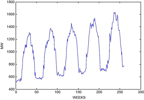
Fig. 1 shows the maximum transfer power values for the whole five years (years 2000–2004). It is clear from the results that the variation of the maximum power transfer values, which is recorded weekly, that is narrow enough to assume as a practical hypothesis with a constant value of maximum transfer power. Also the figure indicates that the demand on the power is increasing by approximately 6.7% every year. Furthermore, the maximum load for each year occurs in the months of July and August.

Figure 1 Illustrates the maximum transfer power values for the years (2000–2004).

Fig. 2 it is a graphical comparison of the first realization of the approximate and the exact secondary conditional standard deviations, which reveals the distinction between automatically generated and user-specified pre sample data. The results in Fig. 2 were found as follows: First the system data uses automatically generated pre-sample data to gather the approximate residuals and conditional standard deviation processes, and then uses explicitly specified pre-sample data to gather the exact residuals and conditional standard deviation processes. The system data are finally used to compare the approximate conditional standard deviation processes with exact conditional standard deviations processes. Notice that the approximate and exact standard deviations are asymptotically identical. The only difference between the two curves is attributable to the transients induced by the default initial conditions. Although the figure highlights the first realization of conditional standard deviations and the comparison holds for any realization and for the inferred residuals as well.

Figure 2 Graphical comparison of the first realization of the approximate and the exact secondary conditional standard deviations.

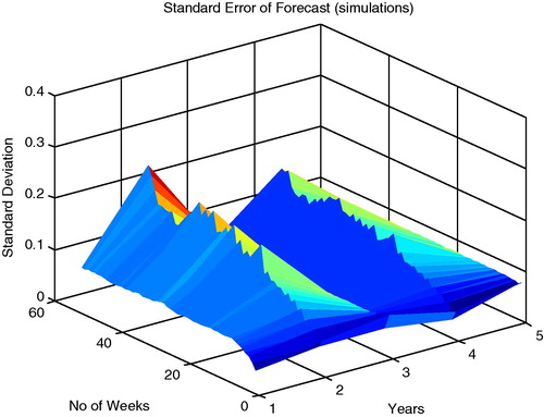
Figs. 3 4 5 6 7 8 9 10 compare the forecast and simulation results on a weekly and yearly bases. Figs. 3 and 4 show the standard deviations of the residuals. These figures show conditional standard deviations of future innovations on a per-period basis. The result represents the standard deviations derived from the minimum mean square error (MMSE) forecasts associated with the recursive volatility model that defines forecast by applying iterate conditional expectation to the conditional mean and variance models, one forecasts period at a time. Since these models are generally recursive in nature, they often require pre-sample data to initiate the iterative processes.

Figure 3 The conditional standard deviations of future originality, from the forecasts results.

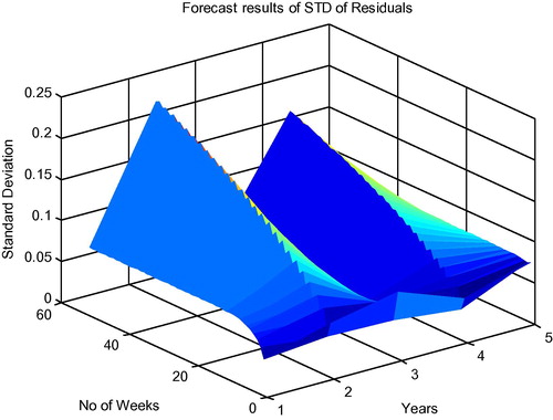
Figure 4 The first forecast output, the conditional standard deviations of future originality, with its counterpart derived from the Monte Carlo simulation.

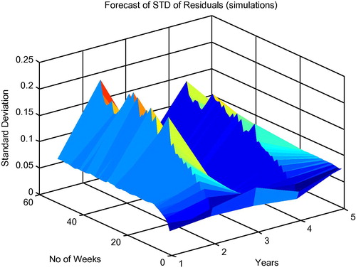
Figure 5 The minimum mean square error forecasts of the conditional mean of the Kingdom of Bahrain reserves power series.

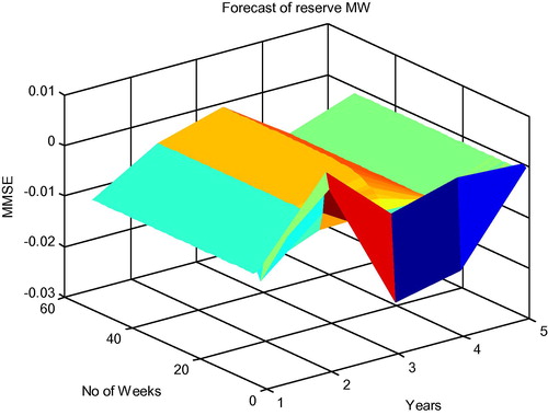
Figure 6 The minimum mean square error forecasts of the conditional mean of the Kingdom of Bahrain reserves power series, with its counterpart derived from the Monte Carlo simulation.

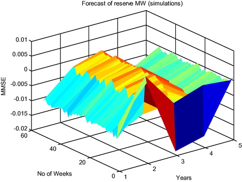
Figure 7 Cumulative holding period power reserves.

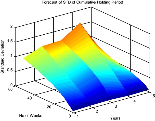
Figure 8 Cumulative holding period power reserves, with its counterpart derived from the Monte Carlo simulation.

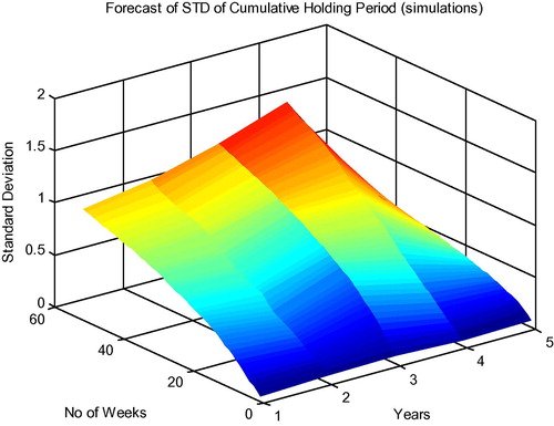
Figure 9 The root mean square errors of the forecasted power reserves.

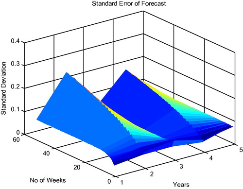
Figure 10 The root mean square errors of the forecasted power reserves, with its counterpart derived from the Monte Carlo simulation.

The system explicitly specifies the needed pre-sample data. It uses the contingent residuals and standard deviations which are estimated by the model as the pre-sample inputs. It uses the Bahrain load forecasts return series as the pre-sample input. In this context, referred to as dependent path simulation, all simulated sample paths share a common conditioning set and evolve from the same set of initial conditions, thus enabling Monte Carlo simulation of forecasts and forecast error distribution.

For this application of Monte Carlo simulation, the system generates a relatively large number of realizations or sample paths, so that it can aggregate across realizations.

It is very clear that forecast and simulation results follow a similar pattern. Figs. 5 and 6 are the comparison of the minimum mean square error. Each element of these figures are associated with the forecasted data. Therefore, each clement is the conditional standard deviation of the corresponding forecast error. By using computed data of MMSE forecasts of the conditional mean and the standard error of the corresponding forecasts, we considered approximate confidence intervals for conditional mean forecasts, with the appreciation becoming more accurate during period of relatively stable volatility. Figs. 7 and 8 are the presentation of the cumulative holding period power reserves. It is again clear that the difference between the figures is insignificant. Figs. 9 and 10 show the comparison of the root mean square errors of the forecasted power reserves. The two figures are viewing exact in shape and they are following each other. These figures show a volatility forecast of returns over multi-period holding in intervals.

4 Conclusion

This study discusses the basic variables and their variation effect by Monte Carlo simulation. The variation of load is the most basic and important aspect of the Monte Carlo simulation method. The results obtained from the first realization of the approximate and the exact secondary conditional standard deviations reveal the similarity between automatically generated and user-specified pre sample data. This reflects the accuracy of the Monte Carlo simulation. It is also seen that that the approximate and exact standard deviations are asymptotically identical. The forecasted loads and the results obtained through the simulation are almost identical.

References

- S. Conti S. Raiti Probabilistic load flow using Monte Carlo techniques for distribution networks with photovoltaic generators Solar Energy 81 12 2007 1473 1481
- Yi Ding P. Wang L. Goel R. Billinton R. Karki Reliability assessment of restructured power systems using reliability network equivalent and pseudo-sequential simulation techniques Electric Power Systems Research 77 12 2007 1665 1671
- G.S. Fishman Monte Carlo: Concepts, Algorithms and Applications 1996 Springer-Verlag New York
- M. Matsumoto T. Nishimura Merenne twister: A623-dimensionally equidistributed uniform pseudorandom number generator ACM Transactions on Modeling and Computer Simulation 8 1 1998 3 30
- Mooney, C.Z., 1997. Monte Carlo Simulation, International Educational and Professional Publication, Thousand Oaks, London, New Delhi, Newbury Park, Sage Publications, CA, Series No. 07-116.
- A. Poulin M. Dostie M. Fournier S. Sansregret Load duration curve: a tool for technico-economic analysis of energy solutions Energy and Buildings 40 1 2007 29 35
- M.R. Qader I.S. Qamber Monte Carlo simulation usage: Kingdom of Bahrain load prediction IETECH Journal of Electrical Analysis 1 2 2007 83 86
- Dong-Joon Shin J.O. Kim K.H. Kim C. Singh Probabilistic approach to available transfer capability calculation Electric Power Systems Research 77 2007 813 820
- R.A. Skeffington P.G. Whitehead E. Heywood J.R. Hall R.A. Wadsworth B. Reynolds Estimating uncertainty in terrestrial critical loads and their exceedances at four sites in the UK International Journal Science of the Total Environment 382 2007 199 213
- N. Yang C.W. Yu F. Wen C.Y. Chung et-al An investigation of reactive power planning based on chance constrained programming International Journal of Electrical Power and Energy Systems 29 9 2007 650 656